MANOVA using Python (using statsmodels and sklearn)
This article explains how to perform the one-way MANOVA in Python. You can refer to this article to know more about MANOVA, when to use MANOVA, assumptions, and how to interpret the MANOVA results.
One-way (one factor) MANOVA in Python
MANOVA example dataset
Suppose we have a dataset of various plant varieties (plant_var) and their associated phenotypic measurements for
plant heights (height) and canopy volume (canopy_vol). We want to see if plant heights and canopy volume are
associated with different plant varieties using MANOVA.
Load dataset,
import pandas as pd
df=pd.read_csv("https://reneshbedre.github.io/assets/posts/ancova/manova_data.csv")
df.head(2)
  plant_var  height  canopy_vol
0         A    20.0         0.7
1         A    22.0         0.8
Summary statistics and visualization of dataset
Get summary statistics based on each dependent variable,
from dfply import *
# summary statistics for dependent variable height
df >> group_by(X.plant_var) >> summarize(n=X['height'].count(), mean=X['height'].mean(), std=X['height'].std())
# output
  plant_var   n   mean       std
0         A  10  18.90  2.923088
1         B  10  16.54  1.920185
2         C  10   3.05  1.039498
3         D  10   9.35  2.106735

# summary statistics for dependent variable canopy_vol
df >> group_by(X.plant_var) >> summarize(n=X['canopy_vol'].count(), mean=X['canopy_vol'].mean(), std=X['canopy_vol'].std())
# output
  plant_var   n   mean       std
0         A  10  0.784  0.121308
1         B  10  0.608  0.096816
2         C  10  0.272  0.143279
3         D  10  0.474  0.094540
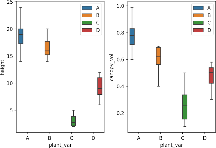
Visualize dataset,
import seaborn as sns
import matplotlib.pyplot as plt
fig, axs = plt.subplots(ncols=2)
sns.boxplot(data=df, x="plant_var", y="height", hue=df.plant_var.tolist(), ax=axs[0])
sns.boxplot(data=df, x="plant_var", y="canopy_vol", hue=df.plant_var.tolist(), ax=axs[1])
plt.show()
perform one-way MANOVA
from statsmodels.multivariate.manova import MANOVA
fit = MANOVA.from_formula('height + canopy_vol ~ plant_var', data=df)
print(fit.mv_test())
# output
                  Multivariate linear model
==============================================================

--------------------------------------------------------------
       Intercept         Value  Num DF  Den DF F Value  Pr > F
--------------------------------------------------------------
          Wilks' lambda  0.0374 2.0000 35.0000 450.0766 0.0000
         Pillai's trace  0.9626 2.0000 35.0000 450.0766 0.0000
 Hotelling-Lawley trace 25.7187 2.0000 35.0000 450.0766 0.0000
    Roy's greatest root 25.7187 2.0000 35.0000 450.0766 0.0000
--------------------------------------------------------------

--------------------------------------------------------------
       plant_var         Value  Num DF  Den DF F Value  Pr > F
--------------------------------------------------------------
          Wilks' lambda  0.0797 6.0000 70.0000  29.6513 0.0000
         Pillai's trace  1.0365 6.0000 72.0000  12.9093 0.0000
 Hotelling-Lawley trace 10.0847 6.0000 44.9320  58.0496 0.0000
    Roy's greatest root  9.9380 3.0000 36.0000 119.2558 0.0000
==============================================================
The Pillai’s Trace test statistics is statistically significant [Pillai’s Trace = 1.03, F(6, 72) = 12.90, p < 0.001] and indicates that plant varieties has a statistically significant association with both combined plant height and canopy volume.
post-hoc test
Here we will perform the linear discriminant analysis (LDA) using sklearn to see the differences between each group.
LDA will discriminate the groups using information from both the dependent variables.
from sklearn.discriminant_analysis import LinearDiscriminantAnalysis as lda
X = df[["height", "canopy_vol"]]
y = df["plant_var"]
post_hoc = lda().fit(X=X, y=y)

# get Prior probabilities of groups:
post_hoc.priors_
array([0.25, 0.25, 0.25, 0.25])

# get group means
post_hoc.means_
array([[18.9  ,  0.784],
       [16.54 ,  0.608],
       [ 3.05 ,  0.272],
       [ 9.35 ,  0.474]])

# get Coefficients of linear discriminants
post_hoc.scalings_
array([[-0.43883736, -0.2751091 ],
       [-1.39491582,  9.32562799]])

# get Proportion of trace (variance explained by each of the selected components)
post_hoc.explained_variance_ratio_
array([0.98545382, 0.01454618])

# plot
X_new = pd.DataFrame(lda().fit(X=X, y=y).transform(X), columns=["lda1", "lda2"])
X_new["plant_var"] = df["plant_var"]
sns.scatterplot(data=X_new, x="lda1", y="lda2", hue=df.plant_var.tolist())
plt.show()
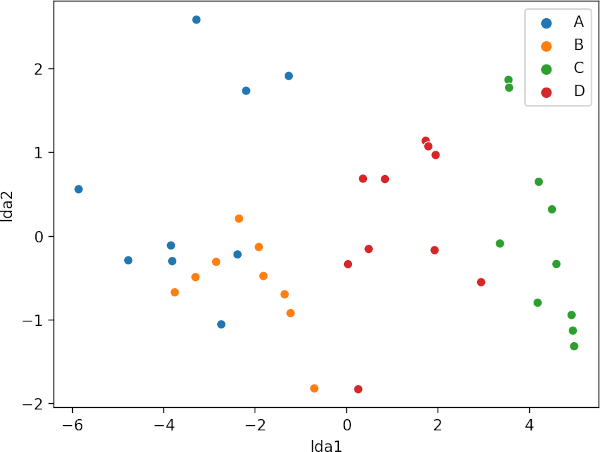
The LDA scatter plot discriminates against multiple plant varieties based on the two dependent variables. The C and D plant variety has a significant difference (well separated) as compared to A and B. A and B plant varieties are more similar to each other. Overall, LDA discriminated between multiple plant varieties.
Read detail about MANOVA here
If you have any questions, comments or recommendations, please email me at reneshbe@gmail.com
This work is licensed under a Creative Commons Attribution 4.0 International License

