Two-Way ANOVA in R: How to Analyze and Interpret Results
Two-way ANOVA (Analysis of Variance) is a statistical method for analyzing the effect of two independent variables on a dependent (response) variable.
Two-way ANOVA is also known as two-factor ANOVA because it involves two independent variables (factor or group variables).
You can use built-in function aov() function
to perform two-way ANOVA in R.
The general syntax of aov() function is:
# fit ANOVA model
model <- aov(y ~ x1 + x2 + x1:x2,  data = df)

# view ANOVA summary
summary(model)
Where,
| Parameter | Description | |
|---|---|---|
y |
Dependent variable (should be continuous variable) | |
x1 |
First independent variable (should be categorical variable) | |
x2 |
Second independent variable (should be categorical variable) | |
x1:x2 |
Interaction between two independent variables |
The following comprehensive example illustrates how to use two-way ANOVA for analyzing group differences (main effects) and interaction effects. As you read this post, you will gain a deeper understanding of two-way ANOVA and its practical applications.
How to Perform Two-Way ANOVA in R
For example, a researcher wants to analyze the effect of plant genotypes and locations on the plant height. The researcher collects the data of four genotypes from three different locations and measure plant height.
The researcher wants to test the following null hypotheses:
Null Hypothesis 1: The plant height is equal among plant genotypes i.e. the mean of plant height is equal
Null Hypothesis 2: The plant height is equal at different locations i.e. the mean of plant height is equal
Null Hypothesis 3: There is no significant effect of plant genotypes and location on the height of the plants i.e. there
is no significant interaction effect
Here, the alternative hypothesis is two-sided as the plant height can be lesser or greater for individual independent variables or for their interaction.
Load and view the dataset,
# load dataset
df <- read.csv("https://reneshbedre.github.io/assets/posts/anova/two_way_anova.csv")

# view five rows of data frame
head(df)

  genotype location height
1        A       L1      5
2        A       L1      6
3        A       L1      7
4        A       L2      7
5        A       L2      7
6        A       L2      6
Check descriptive statistics (mean and variance) for each plant genotype and location,
# load package
library(dplyr)

# get descriptive statistics
df  %>% group_by(genotype, location) %>% summarise(mean = mean(height), var = var(height))

# A tibble: 9 × 4
# Groups:   genotype [3]
  genotype location  mean   var
  <chr>    <chr>    <dbl> <dbl>
1 A        L1        6    1
2 A        L2        6.67 0.333
3 A        L3       11    1
4 B        L1        7.67 2.33
5 B        L2       10    1
6 B        L3       15    1
7 C        L1        5.67 0.333
8 C        L2        7.33 0.333
9 C        L3       15.7  1.33
Visualize the box plot
# load package
library("ggplot2")

# create boxplot
ggplot(df, aes(x = factor(genotype), y = height, fill = location)) +
    geom_boxplot() +
    geom_point(aes(fill = location), size = 4, shape = 21,
               position = position_jitterdodge())
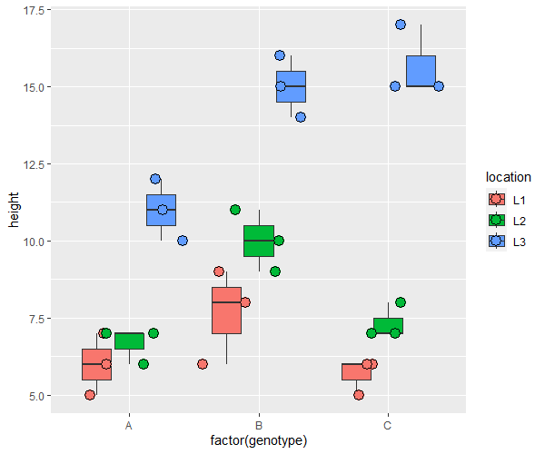
From the box plot and descriptive statistics, we can see that plant height is greatly differ by genotype and location.
Now, we will perform a two-way ANOVA to check whether these differences in plant height are statistically significant and if there is a significant interaction effect between genotype and location.
Perform a two-way ANOVA and summarise the results using summary() function,
# fit model
model <- aov(height ~ genotype + location + genotype:location, data = df)

# summary statistics
summary(model)

                  Df Sum Sq Mean Sq F value   Pr(>F)
genotype           2  40.67   20.33   21.11 1.90e-05 ***
location           2 277.56  138.78  144.12 8.38e-12 ***
genotype:location  4  23.11    5.78    6.00    0.003 **
Residuals         18  17.33    0.96
---
Signif. codes:  0 ‘***’ 0.001 ‘**’ 0.01 ‘*’ 0.05 ‘.’ 0.1 ‘ ’ 1
---
Signif. codes:  0 ‘***’ 0.001 ‘**’ 0.01 ‘*’ 0.05 ‘.’ 0.1 ‘ ’ 1
Note: This ANOVA is performed for a balanced design i.e. equal sample size for each group. If you have an unbalanced design, you should perform an ANOVA with type III sums of squares.
The two-way ANOVA analysis reports the following important statistics for main effects and interaction effects,
| Factor | F | p value |
|---|---|---|
| genotype (main effect) | 21.11 | 1.90e-05 |
| location (main effect) | 144.12 | 8.38e-12 |
| genotype:location (interaction effect) | 6.00 | 0.003 |
According to the two-way ANOVA results, the p value is significant [F(2, 18) = 21.11, p < 0.05] for genotype. Hence, we reject the null hypothesis and conclude that plant height among genotypes is significantly different.
Similarly, the p value is significant [F(2, 18) = 144.12, p < 0.05] for location. Hence, we reject the null hypothesis and conclude that location has a significant effect on plant height.
The interaction between plant genotypes and location is also significant [F(4, 18) = 6, p < 0.05]. Hence, we reject the null hypothesis, and conclude that both plant genotypes and location significantly influence plant height.
Relevant article
Enhance your skills with courses on Statistics and R
- Introduction to Statistics
- R Programming
- Data Science: Foundations using R Specialization
- Data Analysis with R Specialization
- Getting Started with Rstudio
- Applied Data Science with R Specialization
- Statistical Analysis with R for Public Health Specialization
This work is licensed under a Creative Commons Attribution 4.0 International License
Some of the links on this page may be affiliate links, which means we may get an affiliate commission on a valid purchase. The retailer will pay the commission at no additional cost to you.

