Decision tree algorithm for classifications (with illustrative example)

Page content

• Decision tree introduction
• Decision tree terminologies and representation
• Decision tree building
  • Tree splitting
  • Stopping criteria
  • Pruning
• Steps involved in decision tree learning
• Decision tree example
• Impurity measures
  • Entropy
  • Information gain (IG)
• How to choose a feature for splitting?
• Decision tree algorithms
  • CART (Classification and Regression Trees)
  • C4.5
  • CHAID (Chi-Squared Automatic Interaction Detection)
  • QUEST (Quick, Unbiased, Efficient, Statistical Tree)
• Advantages of decision tree

Decision tree introduction

The decision tree learning is a supervised machine learning algorithm used in classification and regression analysis. It is a non-parametric method that helps in a developing powerful predictive model (classifier) for the classification of target variables (dependent variable) based on the multiple independent (predictor) variables (also known as input features).

The input features and target variable in the decision tree can be continuous or categorical variables. Decision trees are largely utilized in image processing, medical disease classification, content marketing, remote sensing, web applications, and text classification.

Decision tree terminologies and representation

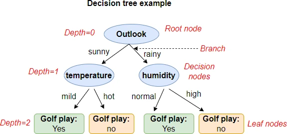
The decision tree is a hierarchical tree-like data structure containing the nodes and hierarchy of branches. The topmost node is called a root node. The root node represent all datasets for features and the root node does not have incoming branches.

The middle incoming nodes are called decision or internal nodes. The decision nodes test the features (sometimes also called attributes) for a target class. There can be multiple decision nodes based on the depth of the decision tree. The down most node is called a leaf node or terminal node, which represents the classification of the target class.

The decision tree depth (or levels) represents the hierarchy of the tree. The root node has a depth of 0, while the leaf node has the maximum depth. The decision tree depth is a handy parameter to decide when to stop splitting the decision tree.

Decision tree building

The building of the decision tree depends on three methods: tree splitting, stopping, and pruning.

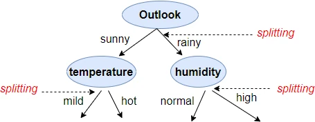
Tree splitting

In tree splitting, the input features are split at the root node or decision nodes to give the terminal node having minimum impurity (i.e. maximum purity - nodes containing a high proportion of correctly classified target class).

Choosing the best feature (also called attribute selection method) is the most crucial part of a decision tree building. Various measures are applied for choosing a feature to split to obtain nodes with minimum impurity. Some of these measures include entropy, information gain, Gini index, etc.

Stopping criteria

The decision tree should be stopped at a certain point, otherwise, the model may overfit, become too complex to interpret, and could be computationally expensive to build. The commonly used stopping criteria for decision building are outlined below

The decision tree should be stopped,

• If the depth of the tree is more than some threshold
• If a specific node gives all correct classifications i.e. node purity is higher than some threshold
• If there is no reduction in node impurity

Pruning

The pruning method is applied when the stopping criteria of the tree do not help. The pruning method involves removing the nodes which do not provide sufficient information. In brief, the decision tree is grown and later pruned to optimize size.

Steps involved in decision tree learning

• Start with the root node with all examples from the training dataset
• Pick the feature with the minimum impurity (highest purity). The impurity measures such as information gain, entropy, and Gini index can be used to identify features with minimum impurity.
• Splitting of the feature which has minimum impurity. This will generate branches of the tree (with decision nodes or terminal nodes)
• Repeat the process and grow the tree until the stopping criteria for the tree are met

Decision tree example

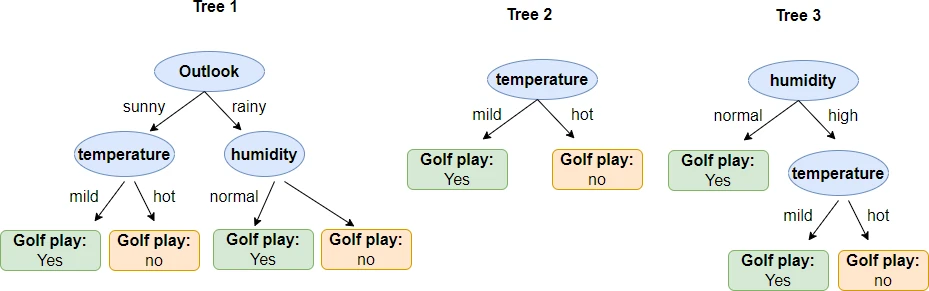
Now, we will construct the decision tree using the golf play example dataset. This golf play example dataset contains three categorical features (outlook, temperature, and humidity) and one target variable (play golf) with two output classes (yes or no).

outlook	temperature	humidity	play golf
rain	hot	high	no
rain	hot	high	no
sunny	mild	high	yes
sunny	mild	normal	yes
rain	hot	high	no
rain	mild	normal	yes
sunny	mild	normal	yes
rain	mild	normal	yes

Table 1: Golf play dataset

Example decision trees based on the golf play dataset (Table 1),

Impurity measures

The selection of appropriate features is essential for the effective splitting of the decision tree. Here, we will discuss in detail how to calculate entropy and information gain as a measure of impurity for the features in decision tree.

Entropy

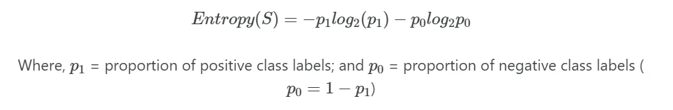
In a decision tree, entropy is a measure of node impurity. The values of entropy range between 0 and 1. The entropy is 0 when all the samples belong to the same class labels. The entropy is 1 when the equal number of samples are found in both class labels. The lower the value of entropy, the better the classification.

Suppose, if there is S sample dataset, then the entropy for S for binary classification (with two class labels) is given as,

For example, the entropy(S) for the golf play dataset (Table 1) is given as,

If there are multiple class labels, then entropy(S) with c class labels is given as,

Information gain (IG)

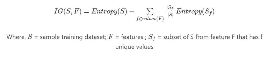
Information gain (IG) for a feature F is a expected reduction in entropy based on the all values of a given feature F. The values of information gain range between 0 and 1. In contrast to entropy, the higher value of information gain is better for classification. The formula for information gain can be written as,

For example, the IG(S, F=outlook) for the Table 1 is given as,

First, calculate the entropy for outlook values (sunny and rainy),

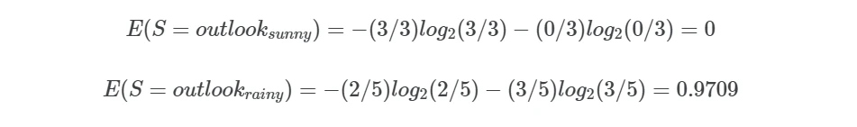
second, calculate the expected entropy for the outlook values (sunny and rainy),

Now, calculate the information gain for outlook feature,

How to choose a feature for splitting?

Now, you have learned how to calculate the information gain. We will use the information gain as impurity measure to choose the feature to split at root node.

In decision tree example, you have seen that there are three possible ways to split the tree at root node. We will use information gain measure to check which feature has maximum purity to split at the node. A node is said to be pure if it gives all correct classifications i.e. it has maximum information gain (close to 1) or minimum entropy (close to 0).

In the above example, we have calculated the information gain for the outlook feature. Similarly, calculate the information gain for temperature and humidity features.

Calculate the entropy,

<img src="/assets/posts/dtree/entropy_cal_features.webp" width="940" height="258" loading="lazy" alt="calculate entropy al \( E(S=temperature_{mild}) = -(5/5)log_2(5/5) - (0/5)log_2(0/5) = 0 \)

\( E(S=temperature_{hot}) = -(0/3)log_2(0/3) - (3/3)log_2(3/3) = 0 \)

\( E(S=humidity_{normal}) = -(4/4)log_2(4/4) - (0/4)log_2(0/4) = 0 \)

\( E(S=humidity_{high}) = -(1/4)log_2(1/4) - (3/4)log_2(3/4) = 0.8112 \)

–>

Calculate the information gain (IG),

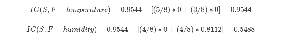
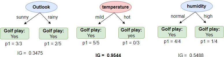
Among the three features, the temperature has the maximum information gain (IG = 0.9544), and therefore, the temperature is the best feature to split at the root node.

Similarly, you can iterate over to select the feature with the highest information for a child node of the previous nodes. You can grow the tree until the stopping criteria are met.

Decision tree algorithms

The CART (Classification and Regression Trees), C4.5, CHAID (Chi-Squared Automatic Interaction Detection), and QUEST (Quick, Unbiased, Efficient, Statistical Tree) are some of the commonly used algorithms used for building the decision tree. The decision tree algorithms can be forward (tree-growing) and backward (tree-pruning).

CART (Classification and Regression Trees)

The CART builds the tree using the backward (tree-pruning) approach. CART is a greedy algorithm which first grows the large tree by greedy splitting and prune it later to the optimum size.

The CART uses the Gini index as an impurity measure to choose the features for splitting. Both input features and output target variables can be categorical or continuous. CART builds the binary tree i.e. the split has two branches.

C4.5

C4.5 is an improved version of ID3 (Iterative Dichotomiser 3). The C4.5 uses the information gain or gain ratios as an impurity measure to choose the features for splitting. Both input features and output target variables can be categorical or continuous.

CHAID (Chi-Squared Automatic Interaction Detection)

The CHAID uses the Chi-Squared statistics to choose the features for splitting. The input features should be categorical or continuous, and the output target variable must be categorical. The CHAID can split the node with more than two branches.

QUEST (Quick, Unbiased, Efficient, Statistical Tree)

The QUEST uses the statistical significance tests such as Chi-Squared and ANOVA methods to choose the features for splitting. The input features should be categorical or continuous, and the output target variable must be categorical. Unlike CHAID, splits are binary (only two branches) in QUEST.

Advantages of decision tree

• Decision trees are simple classifiers which easy to understand and interpret
• Decision tree can be used for classifying categorical and continuous data i.e. decision tree can be applied for both classification and regression analysis
• Decision tree is a non-parametric method and hence does not depend on underlying data distribution
• Decision tree algorithms can automatically select the features for best classification and hence no need to explicitly perform feature selection
• Decision tree models are highly accurate if trained on high-quality datasets

Enhance your skills with courses on machine learning

• Advanced Learning Algorithms
• Machine Learning Specialization
• Machine Learning with Python
• Machine Learning for Data Analysis
• Supervised Machine Learning: Regression and Classification
• Unsupervised Learning, Recommenders, Reinforcement Learning
• Deep Learning Specialization
• AI For Everyone
• AI in Healthcare Specialization
• Cluster Analysis in Data Mining

References

1. Song YY, Ying LU. Decision tree methods: applications for classification and prediction. Shanghai archives of psychiatry. 2015 Apr 4;27(2):130.
2. Alsagheer RH, Alharan AF, Al-Haboobi AS. Popular decision tree algorithms of data mining techniques: a review. International Journal of Computer Science and Mobile Computing. 2017 Jun;6(6):133-42.
3. Krzywinski M, Altman N. Classification and regression trees. Nature Methods. 2017 Jul 28;14(8):757-8.

If you have any questions, comments or recommendations, please email me at reneshbe@gmail.com

This work is licensed under a Creative Commons Attribution 4.0 International License

Some of the links on this page may be affiliate links, which means we may get an affiliate commission on a valid purchase. The retailer will pay the commission at no additional cost to you.