How to Conduct Durbin-Watson Test in R
Durbin-Watson (DW) test
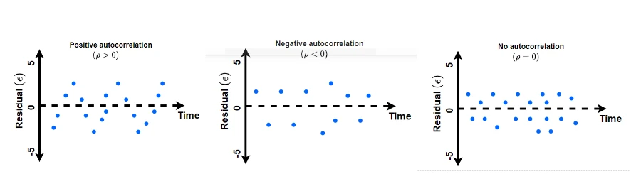
- Durbin-Watson (DW) test is used for analyzing the first-order autocorrelation (also known as serial correlation) in ordinary least square (OLS) regression analysis in time series dataset i.e. residuals are independent of one time to its prior time. First-order autocorrelation is a correlation between the successive (present and prior) residuals for the same variable.
- Durbin-Watson test is commonly used on time series dataset (e.g. events measured on different periods) as time series dataset tends to exhibit positive autocorrelation.
- The value of autocorrelation can range from -1 to 1, where -1 to 0 range represents negative autocorrelation whereas the range 0 to 1 represents positive autocorrelation.
Durbin-Watson test Hypotheses and statistics
Durbin-Watson test analyzes the null hypothesis that residuals from the regression are not autocorrelated (autocorrelation coefficient, ρ = 0) versus the alternative hypothesis that residuals from the regression are positively autocorrelated (autocorrelation coefficient, ρ > 0)
Durbin-Watson test statistics d is given as,
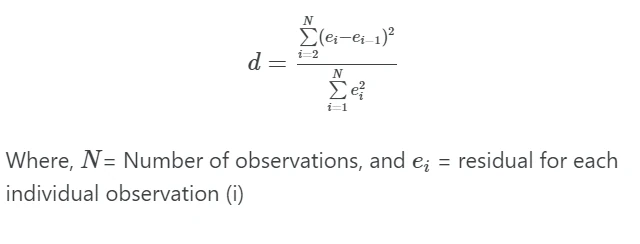
Durbin-Watson test statistics (d) ranges from 0 to 4 and see following table for Durbin-Watson test statistic interpretation,
| d | Interpretation |
|---|---|
| d = 2 | No autocorrelation (ρ = 0) |
| d < 2 (d = 0) | positive autocorrelation (perfect positive autocorrelation i.e. ρ = +1) |
| d > 2 (d = 4 ) | negative autocorrelation (perfect negative autocorrelation i.e. ρ = -1) |
In practice, if the d is in between 1.5 and 2.5, it indicates there is no autocorrelation. If d < 1.5, it indicates positive autocorrelation, whereas if d > 2.5, it indicates negative autocorrelation.
The Durbin-Watson test p value depends on the Durbin-Watson statistic (d) value, the number of independent variables (k) in the regression, and the total number of observations (N).
In terms of Durbin-Watson critical values table, if d < lower critical value (dL), reject the null hypothesis, whereas if d > upper critical value (dU), fail to reject null hypothesis. The region between dL and dU is inconclusive.
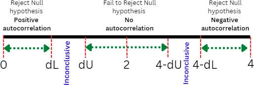
If d < dL, indicates a significantly small p value (say p < 0.05) and implies substantial positive autocorrelation within the residuals. In contrast, if d > dU then p value is larger (say p > 0.05), we fail to reject the null hypothesis and conclude that residuals are not autocorrelated. If d is substantially larger than 2, you should also test the hypothesis for negative autocorrelation.
Learn more about hypothesis testing and interpretation
Perform Durbin-Watson test in R
We will use the tidyverse, stats, and lmtest R packages for this tutorial.
Dataset
Suppose, we have a hypothetical time series dataset consisting of company stock price over a period of 12 months. You can
import your dataset using read_csv() function available in tidyverse package.
# R version 4.1.2 (2021-11-01)
library(tidyverse)
df = read_csv("https://reneshbedre.github.io/assets/posts/reg/stock_price.csv")
head(df, 2)
# output
  months stock_price
   <dbl>       <dbl>
1      1         122
2      2         129
Check out other ways to import CSV datasets in R
Fit the regression model
Fit the regression model with months as independent variables and stock_price as the dependent variable,
library(stats)
model <- lm(formula = stock_price ~ months, data = df)

model
# output
Call:
lm(formula = stock_price ~ months, data = df)

Coefficients:
(Intercept)       months
     114.61         5.92
Learn more about regression analysis
Calculate Durbin-Watson (DW) test in R
We will use dwtest() function avialble in lmtest R package for performing the Durbin-Watson (DW) test. The dwtest()
function takes the fitted regression model and returns DW test statistics (d) and p value.
library(lmtest)
dwtest(formula = model,  alternative = "two.sided")

# output

	Durbin-Watson test

data:  model
DW = 2.5848, p-value = 0.4705
alternative hypothesis: true autocorrelation is not 0
In the Durbin-Watson critical values table, the critical region lies between 0.97 (dL) and 1.33 (dU) for N=12 at 5% significance. Since the Durbin-Watson test statistic (DW=2.58) is higher than 1.33 (DW > dU), we fail to reject the null hypothesis (p > 0.05) that there is no autocorrelation.
As the p value obtained from the Durbin-Watson test is not significant (d = 2.584, p = 0.470), we fail to reject the null hypothesis. Hence, we conclude that the residuals are not autocorrelated.
Check how to perform Durbin-Watson in Python
Enhance your skills with statistical courses using R
- Introduction to Statistics
- Understanding Clinical Research: Behind the Statistics
- Statistics with R Specialization
- Data Science: Foundations using R Specialization
References
- Salamon SJ, Hansen HJ, Abbott D. How real are observed trends in small correlated datasets?. Royal Society open science. 2019 Mar 20;6(3):181089.
- Turner SL, Forbes AB, Karahalios A, Taljaard M, McKenzie JE. Evaluation of statistical methods used in the analysis of interrupted time series studies: a simulation study. BMC medical research methodology. 2021 Dec;21(1):1-8.
- Durbin-Watson
If you have any questions, comments, corrections, or recommendations, please email me at reneshbe@gmail.com
This work is licensed under a Creative Commons Attribution 4.0 International License
Some of the links on this page may be affiliate links, which means we may get an affiliate commission on a valid purchase. The retailer will pay the commission at no additional cost to you.

