Kaplan-Meier Survival Analysis in R
Survival analysis (also known as time-to-event analysis) is a statistical method for analyzing the duration of time until the event of interest occurs (e.g. death of patients).
The Kaplan-Meier survival method is a non-parametric statistical technique that estimates the survival probability of an event occurring at various points in survival time.
In the Kaplan-Meier survival curve, survival probability is plotted against survival time. The survival curve is useful for understanding the median survival time (the time at which survival probability is 50%).
The Kaplan-Meier survival method is a non-parametric statistical technique that estimates the survival probability of an event occurring at various points in survival time.
The Kaplan-Meier curve is primarily used for descriptive analysis of survival data. When the predictor variable is binary, Kaplan-Meier survival analysis is applied. It does not consider additional predictors in the analysis. A regression-based Cox proportional hazards model (CPH) should be used if you have other continuous variables to study the impact on survival analysis.
This tutorial explains how to perform Kaplan–Meier survival analysis in R.
Getting the dataset
We will use the patient survival data for performing the Kaplan–Meier survival analysis.
Load the dataset,
# load package
# install.packages("tidyverse")
library(tidyverse)

# load data file
df <- read_csv("https://reneshbedre.github.io/assets/posts/survival/survival_data.csv")

# view first few rows
head(df, 5)
# A tibble: 5 × 5
  patient survival_time_days outcome treatment age_years
    <dbl>              <dbl>   <dbl> <chr>         <dbl>
1       1                  1       1 drug_2           75
2       2                  1       1 drug_2           79
3       3                  4       1 drug_2           85
4       4                  5       1 drug_2           76
5       5                  6       0 drug_2           66
This dataset contains 15 patients with their survival times (in days), outcome (1=death, 0=survived), treatments (drug_1 and drug_2), and age of the patients.
Perform Kaplan–Meier survival analysis
In R, the Kaplan–Meier survival analysis can be performed using the Surv() and survfit()
functions from the survival package.
For Kaplan–Meier analysis, you need three key variables i.e. survival time, status at survival time (event of interest), and treatment groups of patients.
First, you need to create a survival object using the Surv() function. In a survival object, the event parameter
must be binary e.g. TRUE/FALSE (TRUE = death), 1/0 (1 = death), 2/1 (2 = death).
# load package
library("survival")

surv = Surv(time = df$survival_time_days, event = df$outcome)

print(surv)
# output
 [1]  1   1   4   5   6+  8   9+  9  12  15+ 22  25+ 37  55  72+
In the above output, the + sign indicates that survival time was censored i.e. patients survived after the time of study, or they have dropped from the study, or they have not followed up the study.
Note: If there are a large number of censored patients in the study, the survival curve may not be reliable. The results should be interpreted cautiously.
Now, we will compute the survival probability for both drug treatments using survfit() function.
fit <- survfit(formula = surv ~ treatment, data = df)
summary(fit)
# output
Call: survfit(formula = surv ~ treatment, data = df)

                treatment=drug_1
 time n.risk n.event survival std.err lower 95% CI upper 95% CI
    8      7       1    0.857   0.132       0.6334            1
   12      6       1    0.714   0.171       0.4471            1
   37      3       1    0.476   0.225       0.1884            1
   55      2       1    0.238   0.203       0.0449            1

                treatment=drug_2
 time n.risk n.event survival std.err lower 95% CI upper 95% CI
    1      8       2    0.750   0.153        0.503        1.000
    4      6       1    0.625   0.171        0.365        1.000
    5      5       1    0.500   0.177        0.250        1.000
    9      3       1    0.333   0.180        0.116        0.961
   22      1       1    0.000     NaN           NA           NA
Create Kaplan–Meier survival curve
Visualize the Kaplan–Meier survival curve for both treatments (drug_1 and drug_2). We will use the ggsurvplot() function
from the survminer package.
# load package
# install.packages("survminer")
library("survminer")

# plot Kaplan–Meier survival curve
ggsurvplot(fit = fit, pval = TRUE, surv.median.line = "hv",
            xlab = "Survival time (Days)", ylab = "Survival probability")

# with confidence interval
ggsurvplot(fit = fit, pval = TRUE, surv.median.line = "hv", conf.int =TRUE,
            xlab = "Survival time (Days)", ylab = "Survival probability")
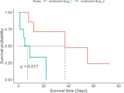
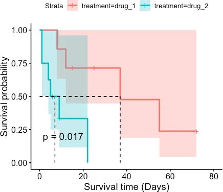
The patient survival rate is higher for drug_1 treatment than for drug_2 treatment. Similarly, the median survival time (time at which survival probability is 50%) is higher for patients taking drug_1 treatment (37 days) than drug_2 treatment (7 days).
Related: Survival analysis
Enhance your skills with courses on Statistics and R
- Introduction to Statistics
- R Programming
- Data Science: Foundations using R Specialization
- Data Analysis with R Specialization
- Getting Started with Rstudio
- Applied Data Science with R Specialization
- Statistical Analysis with R for Public Health Specialization
This work is licensed under a Creative Commons Attribution 4.0 International License
Some of the links on this page may be affiliate links, which means we may get an affiliate commission on a valid purchase. The retailer will pay the commission at no additional cost to you.

