Survival analysis (Kaplan–Meier, Cox proportional hazards, and Log-rank test methods)
Introduction to survival analysis
- Survival analysis (time-to-event analysis) is a collection of statistical methods for analyzing the duration of time (survival time) until the occurrence of the event of interest (e.g. death or relapse).
- Survival time is a follow-up time measured between the defined starting point and occurrence of an event of interest e.g. time from disease diagnosis and death.
- Some patients’ survival times may not be known in survival analysis. This is because not all patients are exposed to the event of interest, and some patients are lost to follow-up before the study period ends. This phenomenon is known as censoring.
- The standard statistical methods can not be applied to analyze survival data as the data is often censored, heavily skewed, and not normally distributed. These features of survival data makes survival analysis unique method and special statistical methods used for survival analysis.
- The main goal of survival analysis is to estimate the survival probability from survival time and assess the effect of any confounding factors on survival time.
- Survival analysis mostly used in cancer studies. In clinical research, the survival analysis is widely used for predicting the time to death.
Common terms in Survival analysis
Two time-dependent functions viz. survival function S(t) and the hazard function h(t) are important terms in survival analysis.
Survival function (survival probability), S(t), refers to a probability of surviving of a patient from the starting time ( e.g. start of diagnosis) to beyond a specific time t. Survival function also known as survivor function.
Hazard function or hazard rate, h(t), refers to the instantaneous rate of occurrence of event of interest given that the patient is survived until that time. The higher value of hazard function represents higher risk of event of interest. The hazard function is a crucial part of Cox proportional hazards (CPH) model (also known as Cox regression).
Survival function represents the probability of not having an event of interest, whereas hazard function represents the probability of an event of interest occurring.
Hazard ratio (HR) is similar to relative risk and is described as the ratio of hazard rate or failure rate in two treatment groups (e.g. treated vs. control group). The HR = 1 indicates that there are no differences between the two groups. HR > 1 indicates that the event of interest is most likely to occur and vice versa.
Methods of survival analysis
Kaplan–Meier method
Kaplan–Meier method is a nonparametric method for survival analysis. It assumes no specific distribution of survival times and does not assume a relationship between survival times and independent variables.
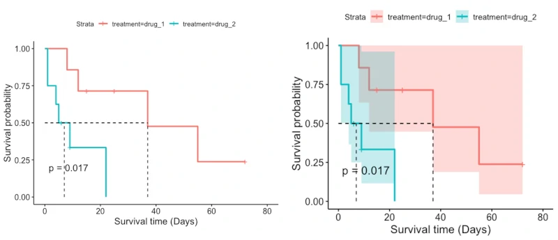
Kaplan–Meier method estimates the survival probability from the observed survival times (both censored and uncensored). Survival probability is plotted against time t in Kaplan–Meier survival curve. The survival curve is useful for understanding the median survival time (time at which survival probability is 50%).
Kaplan–Meier method is suitable for simple survival analysis and does not consider other independent variables (confounding factors) while analyzing survival curves. If there are other confounding factors that you want to include in model, you should use Cox proportional hazards (PH) model (Cox regression).
Kaplan–Meier survival function is given as,
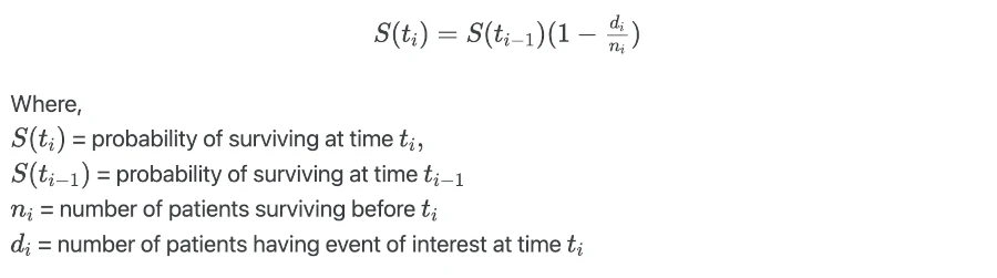
The estimated survival probability only changes at the time (ti) of the event of interest, and it is constant between the two events (ti and ti+1). At time zero (where study begins), the survival probability is 1 (S(0)=1) i.e. all patients are alive at time zero.
The flat survival curve (which is inclined to 1) is good, but vertical survival curve which drops toward 0 is bad (suggest poor survival).
If there are a large number of censored patients in the study, the survival curve may not be reliable. The results should be interpreted cautiously.
Log-rank test
Log-rank test is a nonparametric hypothesis test, which compares two or more survival curves (i.e. survival times for two different condition groups).
The hypothesis for Log-rank test is given as,
Null hypothesis: there are no differences in the survival curves between group1 and group2
Alternate hypothesis: there are differences in the survival curves between group1 and group2
Log-rank test calculates the test statistics by comparing the observed number of events to the expected number of events in underlying condition groups,
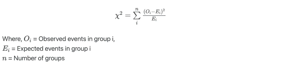
Log-rank test value is compared against the critical value from χ2 distribution with n-1 degree of freedoms
The drawback of Log-rank test is that it does not analyze other independent variables affecting the survival time.
Cox proportional hazards (CPH) model (Cox regression)
Cox proportional hazards (CPH) model is a semiparametric model. It analyzes multiple independent variables for estimating differences between the survival curves. Independent variables can include the variable of interest (e.g. treatments) and other potential confounders (e.g. age of the patients).
CPH model uses the hazard function instead of survival probabilities or survival time. The hazard function is a measure is measure of effect in CPH model.
Hazard ratio (HR) estimates the ratios of hazards in two groups at a particular time and it is given as,
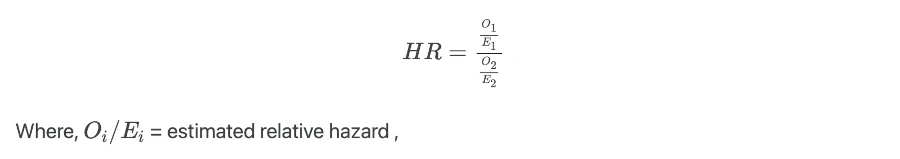
HR is analogous to the odds ratio as in multiple logistic regression analysis. HR is useful in interpreting the results from the Cox proportional hazards (CPH) model.
Assumptions of Cox proportional hazards (CPH) model
- Hazard ratio (HR) is constant over time
- There should be a linear relationship between the log of hazard ratio and independent variables
- The independent variables should be independent of survival times i.e. independent variables should not change with time
Cox proportional hazards (CPH) model
Cox proportional hazards (CPH) model for X independent variables is given as,
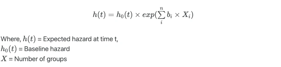
When there is no effect of independent variables (X = 0),

The regression coefficients (bi) are important parameters for explaining the summary of the results. To get regression coefficients (bi) from regression model take log of hazard ratios,
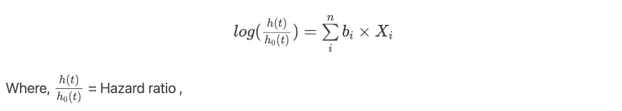
From this function, the quantity exp(bi) is estimated. exp(bi) is the antilog of the
estimated regression coefficient (bi). exp(bi) is also known as the hazard ratio. The regression
coefficient (bi) describes the amount of change in the hazard ratio for one unit change in Xi
whilst all other independent variables are constant.
References
- Bewick V, Cheek L, Ball J. Statistics review 12: survival analysis. Critical care. 2004 Oct;8(5):1-6.
- Clark TG, Bradburn MJ, Love SB, Altman DG. Survival analysis part I: basic concepts and first analyses. British journal of cancer. 2003 Jul;89(2):232-8.
- Schober P, Vetter TR. Survival analysis and interpretation of time-to-event data: the tortoise and the hare. Anesthesia and analgesia. 2018 Sep;127(3):792.
- Singh R, Mukhopadhyay K. Survival analysis in clinical trials: Basics and must know areas. Perspectives in clinical research. 2011 Oct;2(4):1
- Rich JT, Neely JG, Paniello RC, Voelker CC, Nussenbaum B, Wang EW. A practical guide to understanding Kaplan-Meier curves. Otolaryngology—Head and Neck Surgery. 2010 Sep;143(3):331-6.
Related: Kaplan-Meier Survival Analysis in R
Enhance your skills with courses on Statistics and R
- Introduction to Statistics
- R Programming
- Data Science: Foundations using R Specialization
- Data Analysis with R Specialization
- Getting Started with Rstudio
- Applied Data Science with R Specialization
- Statistical Analysis with R for Public Health Specialization
This work is licensed under a Creative Commons Attribution 4.0 International License
Some of the links on this page may be affiliate links, which means we may get an affiliate commission on a valid purchase. The retailer will pay the commission at no additional cost to you.

