Mixed ANOVA using Python and R (with examples)
Mixed ANOVA
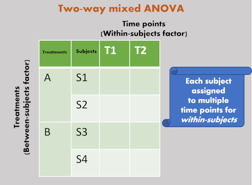
- Unlike independent ANOVA and repeated measures ANOVA, mixed ANOVA has at least two categorical independent variables (factors), one of which is between-subject (each subjects assigned only once to treatment) and the other is within-subject (each subject assigned multiple treatments i.e., time points, before/after treatment, and so on).
- Mixed ANOVA is helpful to understand the interaction effect among between-subject and
within-subject factors, as well as statistical differences among each level in each factor. - Similar to independent ANOVA, mixed ANOVA is omnibus test and does not explicitly tell which specific levels are significantly different from each other in a factor.
Note: mixed ANOVA is also known as mixed factorial ANOVA, mixed design ANOVA, mixed model ANOVA, mixed measures ANOVA, mixed between-within ANOVA
Assumptions of mixed ANOVA
- The responses from subjects (dependent variable) should be continuous
- Residuals (experimental error) are approximately normally distributed for each combination of between-subject and within-subject variable (Shapiro-Wilks Test or histogram)
- Homogeneity of variances or homoscedasticity: There should be equal variance for every level of within-subject factor (Levene’s test)
- Assumption of sphericity: the variances of differences in responses between any two levels of the independent variable (within-subjects factor) should be equal (Mauchly’s test of sphericity). This assumptionn is also known as homogeneity-of-variance-of-differences assumption.
- Homogeneity of the variance-covariance matrices: the pattern of intercorrelation for each level of within-subject variable across between-subject variable should be equal. This is a multivariate version of the Homogeneity of variances. It can be tested using Box’s M test. Box’s M-test has little power and uses a lower alpha level such as 0.001 to assess the p value for significance.
- There should be no significant outlier (this can be checked by boxplot)
Mixed ANOVA example
- Let’s take a simple example of 2 x 2 two-way mixed model ANOVA for better understanding. If you have two plant genotypes (A and B) and would like to compare their yields before (T1) and after (T2) application of fertilizer treatment. Here, plant genotypes and fertilizer application time are two independent variables. Each plant subject receives repeated fertilizer treatment and hence it is within-subject factor. The genotypes of plants is between-subject factor. The yield of the genotypes is dependent variable.
Two-way mixed model ANOVA in Python
In two-way mixed ANOVA, there are two independent variables (between-subject and within-subject) and one dependent variable
Let’s look at how to do a two-way mixed ANOVA in Python,
At the end of article, you can find R notebook for performing two-way mixed ANOVA
Load the dataset
import pandas as pd
df=pd.read_csv("https://reneshbedre.github.io/assets/posts/anova/mixedanova.csv")
df.head(2)
   id genotype  before  after
0   1        A    1.53   4.08
1   2        A    1.83   4.84

# reshape the dataframe in long-format dataframe
df_melt = pd.melt(df.reset_index(), id_vars=['id', 'genotype'], value_vars=['before', 'after'])
#rename column; read more https://www.reneshbedre.com/blog/rename-column-names-pandas.html
df_melt.rename(columns={"variable": "fertilizer", "value": "yield"}, inplace=True)
df_melt.head(2)
   id genotype fertilizer  yield
0   1        A     before   1.53
1   2        A     before   1.83
Read more ways to load a pandas DataFrame
Summarize the dataset
Get summary statistics,
from dfply import *
df_melt >> group_by(X.genotype, X.fertilizer) >> summarize(n=X['yield'].count(), mean=X['yield'].mean(), std=X['yield'].std())

  fertilizer genotype  n   mean       std
0      after        A  5  4.464  0.335306
1     before        A  5  1.592  0.273075
2      after        B  5  5.150  0.778267
3     before        B  5  2.922  0.526802
4      after        C  5  3.194  0.339823
5     before        C  5  2.110  0.099750
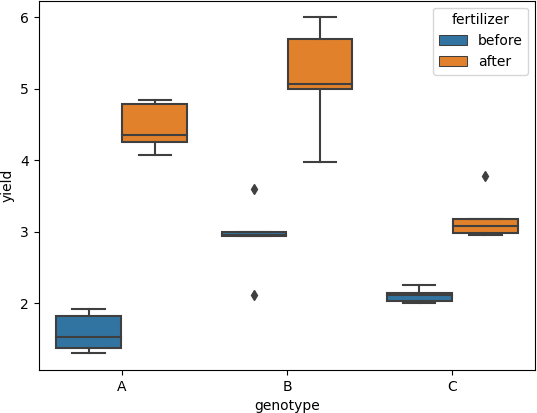
Visualize the dataset using boxplot
boxplot helps detect the differences between different treatments to find any significant outliers
import matplotlib.pyplot as plt
import seaborn as sns
ax = sns.boxplot(x='genotype', y='yield', hue='fertilizer', data=df_melt)
plt.show()
two-way mixed ANOVA
import pingouin as pg
pg.mixed_anova(dv='yield', between='genotype', within='fertilizer', subject='id', data=df_melt)
#output
        Source         SS  DF1  DF2         MS           F         p-unc       np2  eps
0     genotype  10.242987    2   12   5.121493   16.351889  3.741297e-04  0.731566  NaN
1   fertilizer  31.868213    1   12  31.868213  373.404574  2.083410e-10  0.968864  1.0
2  Interaction   4.100347    2   12   2.050173   24.022184  6.371677e-05  0.800148  NaN
Two-way mixed ANOVA estimates the three effects - two main effects and one interaction effect - for statistical significance
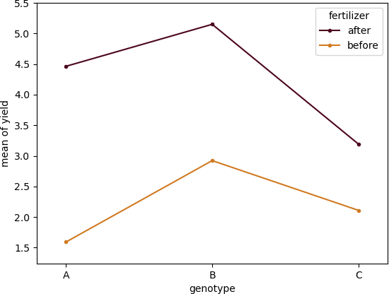
From ANOVA results, the interaction effect between genotype and fertilizer is statistically significant [F(2, 12) = 24.02, p > 0.001, ηp2=0.80]. We conclude that the timing of fertilizer application influence the yield of plant based on genotypes.
we reject the null hypothesis in favor of the alternate hypothesis for genotype (main effect) [F(2, 12) = 16.35, p <0.001, ηp2=0.73]. We conclude that the mean of the yield of plant genotypes differs significantly even we ignore the effect of fertilizer
The main effect for fertilizer is also statistically significant [F(1, 12) = 373.40, p <0.0001, ηp 2=0.96]. We conclude that there is a signifcant difference in yield before and after application of fertilizer even we ignore the effect of genotype.
Note: Generally, it is not appropriate to interpret main effects when interaction is significant.
The measure of effect size (Partial Eta Squared; ηp 2) is higher (0.73, 0.96, and 0.80) for all three effects and suggests that there is a large effect of three effects on a yield of genotypes.
Create a interaction (profile) plot,
from statsmodels.graphics.factorplots import interaction_plot
import matplotlib.pyplot as plt
fig = interaction_plot(x=df_melt['genotype'], trace=df_melt['fertilizer'], response=df_melt['yield'],
    colors=['#4c061d','#d17a22'])
plt.show()
Check mixed ANOVA assumptions
Assumption of sphericity
The assumption of sphericity can be tested using Mauchly’s test of sphericity. The violation of the assumption of sphericity can lead to an increase in type II error (loss of statistical power) and the F value is not valid. This test is not useful here as there are only two levels for within-subjects factor
import pingouin as pg
pg.sphericity(data=df_melt, dv='yield', subject='id', within='fertilizer')[-1]
1.0
As the p value (1.0) is non-significant (p > 0.05), the data met the assumption of sphericity, and variances of differences of independent variable (within-subjects factor) are equal.
Assumption of normality
Shapiro-Wilk test can be used for checking the assumption for normality of each level of the within-subjects factor
df_melt['factor_comb']=df_melt["genotype"] + '-'+df_melt["fertilizer"]
pg.normality(df_melt, dv='yield', group='factor_comb')
                 W      pval  normal
A-before  0.908932  0.461201    True
B-before  0.897502  0.396232    True
C-before  0.956608  0.784187    True
A-after   0.891106  0.362694    True
B-after   0.943001  0.687226    True
C-after   0.779155  0.054206    True
Assumption of homogeneity of variances or homoscedasticity
This assumption can be checked using Levene’s test which is more robust to departure from normality
df_melt_before = pd.melt(df.reset_index(), id_vars=['id', 'genotype'], value_vars=['before'])
df_melt_after = pd.melt(df.reset_index(), id_vars=['id', 'genotype'], value_vars=['after'])
pg.homoscedasticity(df_melt_before, dv='value', group='genotype')
               W     pval  equal_var
levene  1.122517  0.35736       True

pg.homoscedasticity(df_melt_after, dv='value', group='genotype')
              W      pval  equal_var
levene  1.35042  0.295825       True
As the p > 0.05, there is equal variance for each level of within-subject factor
Assumption of Homogeneity of covariances
As there are multiple dependent measures, the homogeneity of variance-covariance matrices formed by the between-subject factor for each level of within-subject should be equal. It can be tested using the Box’s M tests.
Please check R notebook to see the results of Box’s M test
References
- Mixed Model Analysis of Variance
- Vallat, R. (2018). Pingouin: statistics in Python. Journal of Open Source Software, 3(31), 1026, https://doi.org/10.21105/joss.01026
- Two-Way Mixed ANOVA
If you have any questions, comments or recommendations, please email me at reneshbe@gmail.com
This work is licensed under a Creative Commons Attribution 4.0 International License

