Multiple hypothesis testing problem in Bioinformatics
What is multiple testing problem?
- In transcriptomics experiments, we analyze thousands of genes to identify significant differentially expressed genes (DEGs) between two groups (eg. normal vs. treated) which could alter biological mechanisms of a species in response to particular treatment
- In order to identify significant DEGs in terms of fold changes between two groups, it is necessary to apply multiple hypothesis testing (analysis of hypothesis across thousands of genes simultaneously). Each individual hypothesis testing for a single gene involves whether mean of two groups are different or not.
- In multiple hypothesis testing two kinds of errors that need to consider:
Type I error (False positive or chance of making mistake): Null hypothesis is rejected when it is fail to reject (Note: Type I error is also referred as P-value)
Type II error (False negative): Null hypothesis is fail to reject when it is reject - For example, if we want to analyze 10000 genes to identify genes with significant fold changes between two gropus, the probability of getting significant results just due to by chance is 500 (5*10000/100) at a significance level of 0.05 (5%) i.e 500 genes identified as false positive. The number of getting false positives will be more as we test large number of genes (generally in between 20K to 40K in human and plant species). Interpreting false positive results are very harmful as it will lead to wrong conclusions and therefore it is essential to control false positive discovery.
How to minimize false discoveries?
- To control false discoveries from multiple hypothesis testing, it is imperative adjust significance level (α) to reduce the probability of getting Type I error (family-wise error rate or FWER)
-
Family-wise error rate (FWER) is defined as a probability of getting at least one significant result (false discovery) just by chance during multiple testing.
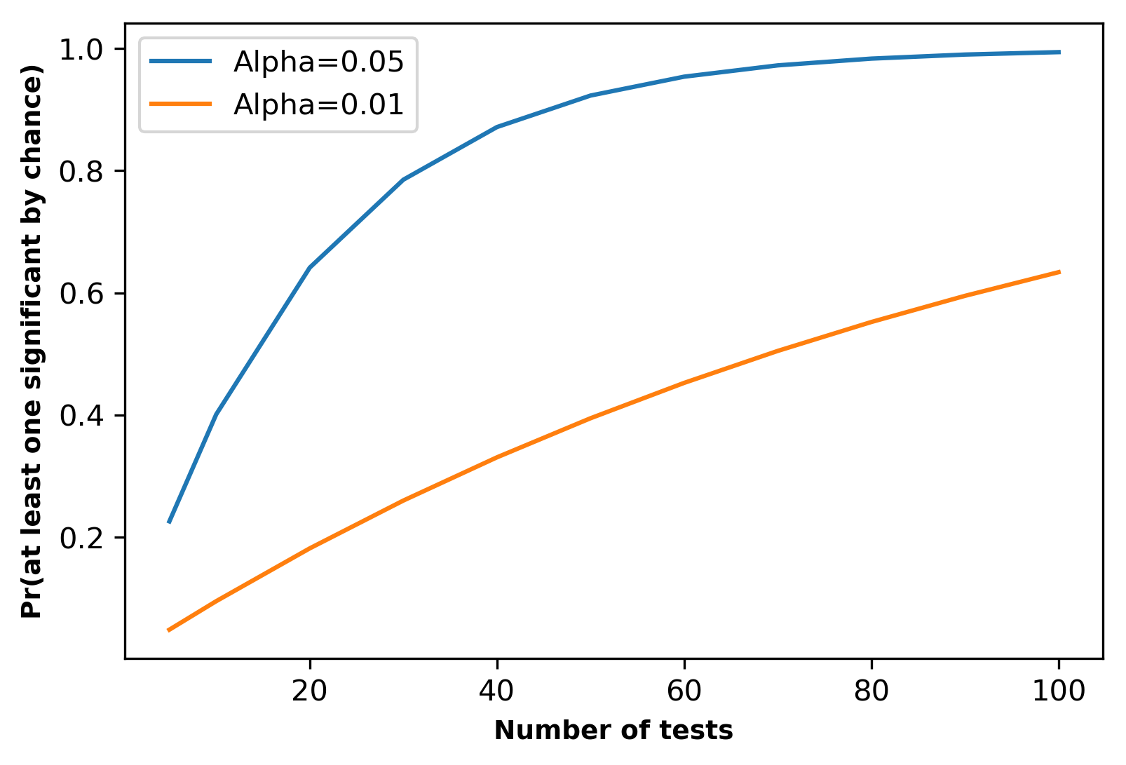
For example, If we perform 50 multiple tests at α=0.05, the probability of getting at least one significant result by chance is ~ 92%
\(P(\text{at least one significant}) = 1−P(\text{no significant)}\)
\(\hspace{114 pt} = 1-(1-0.05)^{50} \sim 0.92\)In transcriptomics experiments, we analyze thousands of genes and therefore, probability of getting false positive results will be much higher.
- FWER can be controlled by using Bonferroni correction where significance level (α) is adjusted to (α/n).
For example, If we perform 50 multiple tests at α=0.05, the probability of getting at least one significant result by chance is ~ 4%
The new adjusted α = 0.05/50 = 0.001
\(P(\text{at least one significant}) = 1−P(\text{no significant)}\)
\(\hspace{114 pt} = 1-(1-0.001)^{50} \sim 0.04\)Caution: Bonferroni correction is a highly conservative method. It can decrease the rate of false positives, but also extremely increases false negatives.
- Another approach to control the false discoveries from multiple hypothesis testing is to control false discovery rate (FDR). FDR is defined as the proportion of false positives among the significant results. Benjamini and Hochberg (1995) technique can be used to control FDR at a specific significance level. Benjamini and Hochberg is more suitable and recommended method for correcting P-values than Bonferroni correction in gene expression analysis.
When not to use multiple hypothesis testing corrections?
p value corrections methods for multiple hypothesis testing can increase the number of false negatives depending on the type of methodology used. If false negative observations are very important or expensive, you should avoid correcting p values during multiple hypothesis testing.
Below graph represents the probability of getting at least one significant result by chance with different numbers tests at α = 0.05 and α = 0.01,
Case study
# load required packages
# make sure you have installed required packages
from scipy.stats import norm
import numpy as np
from statsmodels.stats.multitest import multipletests

# generate 500 random numbers (observations) with mean 0 and standard deviation 1 for
# multiple hypothesis testing
rand_num = norm.rvs(loc=0, scale=1, size=500)
# now, get P-values for these observations using one-sided test
# Alternate hypothesis= observation value is larger than 0
# All observations should fail to reject null hypothesis and any obtained significant
# P-value is just by a chance. We should expect ~25 (5*(500/100) significant P-value
# (at 0.05 significance level) by a chance
pval = 1-norm.cdf(rand_num) # right-sided test
# count P-values < 0.05
# output: 25
print(len(pval[np.where(pval<0.05)]))

# Bonferroni correction
# Get Bonferroni corrected P-value, which is 0.0001
bf_p = 0.05/500
# count P-values < bf_p
# output: 0
print(len(pval[np.where(pval<bf_p)]))

# Benjamini and Hochberg FDR at alpha=0.05
y=multipletests(pvals=pval, alpha=0.05, method="fdr_bh")
# output: 0
print(len(y[1][np.where(y[1]<0.05)]))  # y[1] returns corrected P-vals (array)
If you repeat above code, you should get significant P-values close to 25 which is also referred as Type I error rate
(false positives) and calculated as (25/500=0.05). If you notice, the Type I error rate is equal to P-value
significance level (0.05). After Bonferroni and Benjamini/Hochberg correction, we have obtained 0 false positives
(Type I error rate=0/500=0).
Bonferroni correction to control FWER: False positives = 0
Benjamini and Hochberg to control FDR: False positives = 0
# Now, generate 500 random numbers (observations) with mean 3 and standard deviation 1 for
# multiple hypothesis testing
rand_num = norm.rvs(loc=3, scale=1, size=500)
# now, get P-values for these observations using one-sided test
# Alternate hypothesis= observation value is larger than 0
# All observations should reject null hypothesis (as we are performing cdf with mean=0)
# and any obtained non-significant P-value is just by a chance
pval = 1-norm.cdf(rand_num) # right-sided test
# count P-values < 0.05
# output: 460
print(len(pval[np.where(pval<0.05)]))

# Bonferroni correction
# Get Bonferroni corrected P-value, which is 0.0001
bf_p = 0.05/500
# count P-values < bf_p
# output: 126
print(len(pval[np.where(pval<bf_p)]))

# Benjamini and Hochberg FDR at alpha=0.05
y=multipletests(pvals=pval, alpha=0.05, method="fdr_bh")
# output: 450
print(len(y[1][np.where(y[1]<0.05)]))  # y[1] returns corrected P-vals (array)
If you repeat above code, you should get significant P-values close to 460. The Type II error rate (false negative) is
40/500 = 0.08. After Bonferroni correction, the rate of false negatives is tremendously increased (374/500=0.74),
whereas with Benjamini/Hochberg correction, the rate of false negatives is 50/500 = 0.1.
Bonferroni correction to control FWER: False negatives = 374
Benjamini and Hochberg to control FDR: False negatives = 50
Reference
- Bonferroni CE. Il calcolo delle assicurazioni su gruppi di teste. Studi in onore del professore salvatore ortu carboni. 1935:13-60.
- Benjamini Y, Hochberg Y. Controlling the false discovery rate: a practical and powerful approach to multiple testing. Journal of the royal statistical society. Series B (Methodological). 1995 Jan 1:289-300.
Related reading
If you have any questions, comments or recommendations, please email me at reneshbe@gmail.com
This work is licensed under a Creative Commons Attribution 4.0 International License

