Linear Regression Using Neural Networks (PyTorch)
Introduction and basics of neural networks
- Here, I will use PyTorch for performing the regression analysis using neural networks (NN). PyTorch is a deep learning framework that allows building deep learning models in Python.
- In neural networks, the linear regression model can be written as
\( Y = wX + b \)
Where, \( w \) = weight, b = bias (also known as offset or y-intercept), \( X \) = input (independent variable), and
\( Y \) = target (dependent variable)
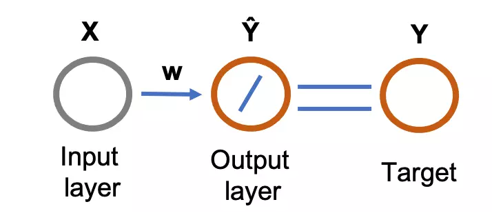
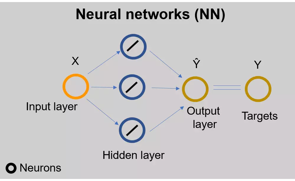
Figure 1: Feed-forward (flows from input to output layer) single-layer neural network for linear regression. The circle represents the neurons. The diagonal line in the output layer represents the linear function (activation function). The output from the neural network (predicted values, \( \hat{Y} \) ) are compared with the target variables to train the network.
Note: Even though neural networks and standard statistical models are alike, their terminologies for representing models are quite different. Check standard statistical model for linear regression.
- The training (learning) of the model is performed to estimate the regression parameters (weights). Linear regression is supervised learning as there is known target associated with the input.
- The training of neural networks is performed using the backpropagation (flows from output to input layer) algorithm.
- The advantage of neural networks over standard statistical analysis is that it is useful when the data does not follow the basic assumption of regression i.e. there is no linear relationship between independent and dependent variables. For this reason, neural networks can be considered as a non-parametric regression model.
- The disadvantage of neural networks is that it does not reveal the significance of the regression parameters. For example, we can perform the hypothesis tests on regression parameters in standard statistical analysis.
Perform Linear Regression with PyTorch
Load the dataset and create tensors
- Load the plant native richness dataset, and create dependent and independent variables as PyTorch tensors.
- Tensor is a specialized data structure similar to the NumPy arrays. The advantage of tensors is that they can be used on graphical processing units (GPUs) to accelerate computing performance. GPUs give higher performance than CPUs.
import torch as th
from bioinfokit.analys import get_data

df = get_data('plant_richness_lr').data
df.head(2)
   ntv_rich      area
0  1.897627  1.602060
1  1.633468  0.477121

# convert variables to PyTorch tensor
X = th.tensor(df[['area']].values, dtype=th.float32)
y = th.tensor(df[['ntv_rich']].values, dtype=th.float32)
Regression model
Create the regression model using th.nn.Linear (PyTorch submodule for NN),
in_features = 1 # number of independent variables
out_features = 1 # dimension of predicted variables
# bias is default true and can be skipped
reg_model = th.nn.Linear(in_features=in_features, out_features=out_features, bias=True)
Loss function
- Define the loss function (also known as cost or error function) to measure the regression error (residuals) between predicted output and actual data (ground truth).
- Mean squared error (MSE), an average squared distance between predicted output and actual data, is used as a loss function in regression.
\( MSE = \frac{\sum_{i=1}^{n}( y_i - \hat{y}_i )^2}{n} \)
Where, \( \hat{y}_i \) = predicted output, \( y_i \) = actual data, n = total patterns (observations)
mse_loss = th.nn.MSELoss()
Gradient descent optimizer
- Now, instantiate a gradient descent optimizer. We use stochastic gradient descent (SGD) optimizer.
- Optimization process aimed at finding regression coefficients (regression parameters) in a such way that loss function is minimum. This error minimization algorithm is also known as the backpropagation of errors.
- The learning rate (
lr) parameter is useful to decide the change in weight that will aim to minimize the loss function. Set a small learning rate. For example, if the model is over-trained (less predictive model), you may getinfloss. In this case, set the learning rate smaller and try again. This is also called hyperparameter tuning.
optimizer = th.optim.SGD(reg_model.parameters(), lr=0.002)
Model training
- Neural networks use iterative solutions to estimate the regression parameters. Reiterate the model multiple times to update the regression parameters until the loss is minimum (it should converge to minimum or zero). This is also known as g radient descent.
# set epoch to 6K
n_epoch = 6000
for i in range(n_epoch):
    # predict model with current regression parameters
    # forward pass (feed the data to model)
    y_pred = reg_model(X)
    # calculate loss function
    step_loss = mse_loss(y_pred, y)

    # Backward to find the derivatives of the loss function with respect to regression parameters
    # make any stored gradients to zero
    # backward pass (go back and update the regression parameters to minimize the loss)
    optimizer.zero_grad()
    step_loss.backward()
    # update with current step regression parameters
    optimizer.step()
    print ('epoch [{}], Loss: {:.2f}'.format(i, step_loss.item()))

# output
epoch [5994], Loss: 0.04
epoch [5995], Loss: 0.04
epoch [5996], Loss: 0.04
epoch [5997], Loss: 0.04
epoch [5998], Loss: 0.04
epoch [5999], Loss: 0.04
Note: It is often difficult to set the required learning rate and the number of epochs to train the neural network model. It is mostly experimental, and you may need to run the model multiple times to tune parameters that led to minimum loss.
Estimate the regression parameters
Now, get the regression parameters from this trained model,
# bias b (offset or y-intercept)
reg_model.bias.item()
1.331221103668213
# weight (w)
reg_model.weight.item()
0.35739263892173767
Regression plot
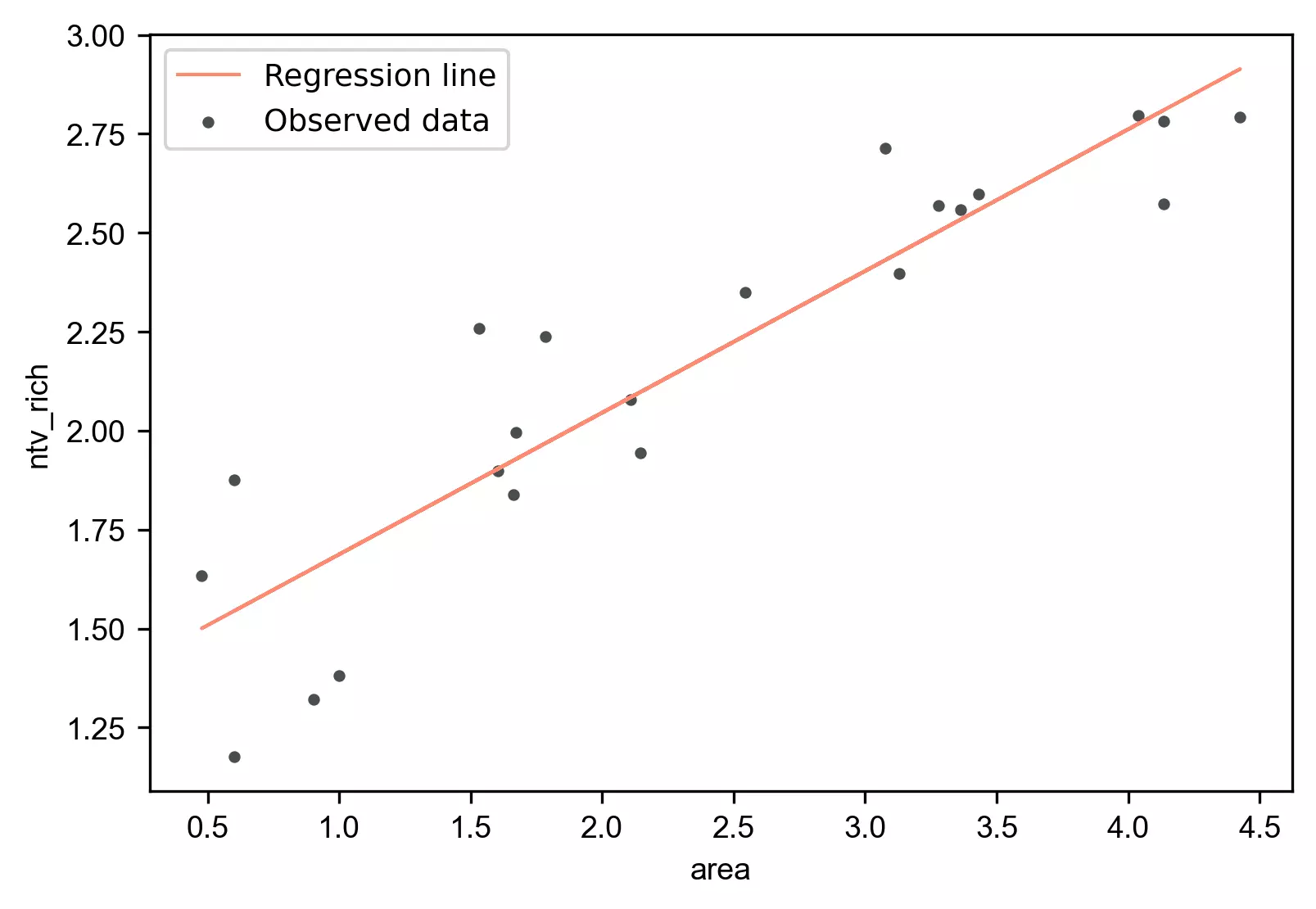
Generate the regression plot,
from bioinfokit.visuz import stat
# detach will not build a gradient computational graph (no backpropagation)
y_pred = reg_model(X).detach()
df['yhat']=y_pred.numpy()
stat.regplot(df=df, x='area', y='ntv_rich', yhat='yhat')
Model performance
Calculate the R-squared to estimate the model performance,
from sklearn.metrics import r2_score
r2_score(y_true=y, y_pred=y_pred.detach().numpy())
0.8276372280771711
Prediction
Now, let’s predict the plant native richness (ntv_rich) from the land area (area),
area = 3
# predict y (ntv_rich) value when X (area) is 3
y_pred = reg_model(th.tensor([[area]], dtype=th.float32)).detach()
y_pred.item()
2.403442859649658
Enhance your skills with courses on regression
- Deep Neural Networks with PyTorch
- Introduction to TensorFlow for Artificial Intelligence, Machine Learning, and Deep Learning
- Machine Learning Specialization
- AI For Everyone
References
- Paszke A, Gross S, Massa F, Lerer A, Bradbury J, Chanan G, Killeen T, Lin Z, Gimelshein N, Antiga L, Desmaison A. Pytorch: An imperative style, high-performance deep learning library. arXiv preprint arXiv:1912.01703. 2019 Dec 3.
- Stevens L, Antiga L, Viehmann T. Deep Learning with PyTorch. Manning Publications
- McMaster RT. Factors influencing vascular plant diversity on 22 islands off the coast of eastern North America. Journal of Biogeography. 2005 Mar;32(3):475-92.
- Paswan RP, Begum SA. Regression and neural networks models for prediction of crop production 1.
This work is licensed under a Creative Commons Attribution 4.0 International License
Some of the links on this page may be affiliate links, which means we may get an affiliate commission on a valid purchase. The retailer will pay the commission at no additional cost to you.

