t-SNE in Python for visualization of high-dimensional data
What is t-Distributed Stochastic Neighbor Embedding (t-SNE)?
t-Distributed Stochastic Neighbor Embedding (t-SNE) is a non-parametric dimensionality reduction technique in which high-dimensional data (n features) is mapped into low-dimensional data (typically 2 or 3 features) while preserving relationship among the data points of original high-dimensional data.
A t-SNE algorithm is an unsupervised machine learning algorithm primarily used for visualizing. Using [scatter plots]((scatter-plot-matplotlib.html), low-dimensional data generated with t-SNE can be visualized easily.
t-SNE is a probabilistic model, and it models the probability of neighboring points such that similar samples will be placed together and dissimilar samples at greater distances. Hence, t-SNE is helpful in understanding the data structure and distribution characteristics of the high-dimensional datasets.
Unlike principal component analysis (PCA) which needs linear data, t-SNE work better with both linear and non-linear well-clustered datasets and produces more meaningful clustering.
Why to use t-SNE?
The majority of big data datasets contain hundreds or thousands of variables. Due to a large number of variables, it is impractical to visualize the data (even with pairwise scatter plots), so we must use dimensional reduction techniques to understand their structure and relationships.
As an example, single-cell RNA-seq (scRNA-seq) produces the expression data for thousands of genes and millions of cells in bioinformatics analysis. To understand biologically meaningful cluster structures, such high-dimensional datasets must be analyzed and visualized.
Interpreting such high-dimensional non-linear data would be impractical without transforming them into low-dimensional data. Using dimension reduction techniques such as t-SNE, high-dimensional datasets can be reduced into two-dimensional space for visualization and understanding biologically meaningful clusters present in high-dimensional datasets.
How to perform t-SNE in Python
In Python, t-SNE analysis and visualization can be performed using the TSNE() function from scikit-learn
and bioinfokit packages.
Here, I will use the scRNA-seq dataset for visualizing the hidden biological clusters. I have downloaded the subset of scRNA-seq dataset of Arabidopsis thaliana root cells processed by 10x genomics Cell Ranger pipeline
This scRNA-seq dataset contains 4406 cells with ~75K sequence reads per cells. This dataset is pre-processed using Seurat R package and only used 2000 highly variable genes (variables or features) for t-SNE visualization.
Now, import the pre-processed scRNA-seq data using get_data() function from bioinfokit package. If you have your
own dataset, you should import it as a pandas dataframe.
# import scRNA-seq as pandas dataframe
from bioinfokit.analys import get_data
df = get_data('ath_root').data
df = df.set_index(df.columns[0])
dft = df.T
dft = dft.set_index(dft.columns[0])
dft.head(2)
# output
gene                AT1G01070  RPP1A  HTR12  AT1G01453  ADF10  PLIM2B  SBTI1.1  GL22  GPAT2  AT1G02570  BXL2  IMPA6  ...  PER72  RAB18  AT5G66440  AT5G66580  AT5G66590  AT5G66800  AT5G66815  AT5G66860  AT5G66985  IRX14H  PER73  RPL26B
AAACCTGAGACAGACC-1       0.51   1.40  -0.26      -0.28  -0.24   -0.14    -0.13 -0.07  -0.29      -0.31 -0.23   0.66  ...  -0.25   0.64       0.61      -0.55      -0.41      -0.43       2.01       3.01      -0.24   -0.18  -0.34    1.16
AAACCTGAGATCCGAG-1      -0.22   1.36  -0.26      -0.28  -0.60   -0.51    -0.13 -0.07  -0.29      -0.31  0.81  -0.31  ...  -0.25   1.25      -0.48      -0.55      -0.41      -0.43      -0.24       0.89      -0.24   -0.18  -0.49   -0.68

# check the dimension (rows, columns)
dft.shape
# output
(4406, 2000)
As there is a very large number of variables (2000), we will use another dimension reduction technique such as PCA to reduce the number of variables to a reasonable number (e.g. 20 to 50) for t-SNE.
Note: The PCA is a recommended method to reduce the number of input features (when there are a large number of features) to a reasonable number (e.g. 20 to 50) to speed up the t-SNE computation time and suppresses the noisy data points.
from sklearn.decomposition import PCA
import pandas as pd

# perform PCA
pca_scores = PCA().fit_transform(dft)
# create a dataframe of pca_scores
df_pc = pd.DataFrame(pca_scores)
Now, perform the t-SNE on the first 50 features obtained from the PCA. By default, TSNE() function uses the Barnes-Hut
approximation, which is computationally less intensive.
# perform t-SNE on PCs scores
# we will use first 50 PCs but this can vary
from sklearn.manifold import TSNE
tsne_em = TSNE(n_components = 2, perplexity = 30.0, early_exaggeration = 12,
               n_iter = 1000, learning_rate = 368, verbose = 1).fit_transform(df_pc.loc[:,0:49])
# output
[t-SNE] Computing 91 nearest neighbors...
[t-SNE] Indexed 4406 samples in 0.081s...
[t-SNE] Computed neighbors for 4406 samples in 1.451s...
[t-SNE] Computed conditional probabilities for sample 1000 / 4406
[t-SNE] Computed conditional probabilities for sample 2000 / 4406
[t-SNE] Computed conditional probabilities for sample 3000 / 4406
[t-SNE] Computed conditional probabilities for sample 4000 / 4406
[t-SNE] Computed conditional probabilities for sample 4406 / 4406
[t-SNE] Mean sigma: 4.812347
[t-SNE] KL divergence after 250 iterations with early exaggeration: 64.164688
[t-SNE] KL divergence after 1000 iterations: 0.840337
# here you can run TSNE multiple times to keep run with lowest KL divergence
Note: t-SNE is a stochastic method and produces slightly different embeddings if run multiple times. t-SNE can be run several times to get the embeddings with the smallest Kullback–Leibler (KL) divergence. The run with the smallest KL could have the greatest variation.
You have run the t-SNE to obtain a run with smallest KL divergenece.
In t-SNE, several parameters needs to be optimized (hyperparameter tuning) for building the effective model.
perplexity is the most important parameter in t-SNE, and it measures the effective number of neighbors. The number of variables in the original high-dimensional data determines the perplexity parameter (standard range 10-100). In case of large, datasets, keeping large perplexity parameter (n/100; where n is the number of observations) is helpful for preserving the global geometry.
In addition to the perplexity parameter, other parameters such as the number of iterations (n_iter), learning rate (set n/12 or 200 whichever is greater), and early exaggeration factor (early_exaggeration) can also affect the visualization and should be optimized for larger datasets (Kobak et al., 2019).
Now, visualize the t-SNE clusters,
# plot t-SNE clusters
from bioinfokit.visuz import cluster
cluster.tsneplot(score=tsne_em)
# plot will be saved in same directory (tsne_2d.png)
Generated t-SNE plot,
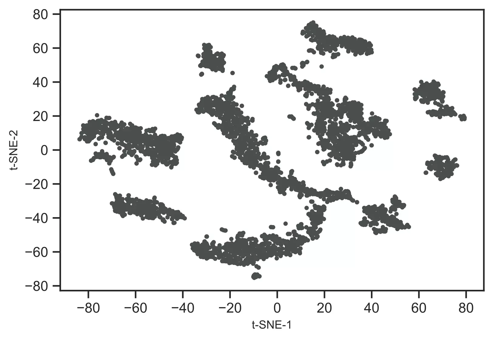
As t-SNE is an unsupervised learning method, we do not have sample target information. Hence, I will recognize the clusters using the DBSCAN clustering algorithm. This will help to color and visualize clusters of similar data points
from sklearn.cluster import DBSCAN
# here eps parameter is very important and optimizing eps is essential
# for well defined clusters. I have run DBSCAN with several eps values
# and got good clusters with eps=3
get_clusters = DBSCAN(eps = 3, min_samples = 10).fit_predict(tsne_em)
# check unique clusters
# -1 value represents noisy points could not assigned to any cluster
set(get_clusters)
# output
{0, 1, 2, 3, 4, 5, 6, 7, 8, 9, 10, 11, 12, -1}
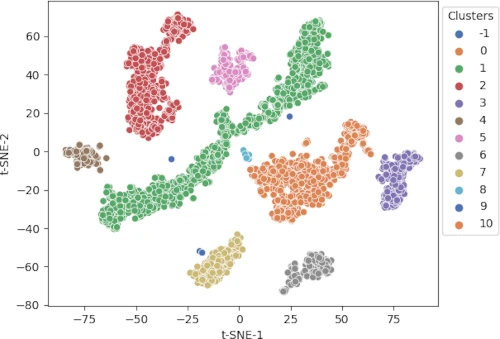
# get t-SNE plot with colors assigned to each cluster
cluster.tsneplot(score=tsne_em, colorlist=get_clusters,
colordot=('#713e5a', '#63a375', '#edc79b', '#d57a66', '#ca6680', '#395B50', '#92AFD7', '#b0413e', '#4381c1', '#736ced', '#631a86', '#de541e', '#022b3a', '#000000'),
legendpos='upper right', legendanchor=(1.15, 1))
Generated t-SNE plot,
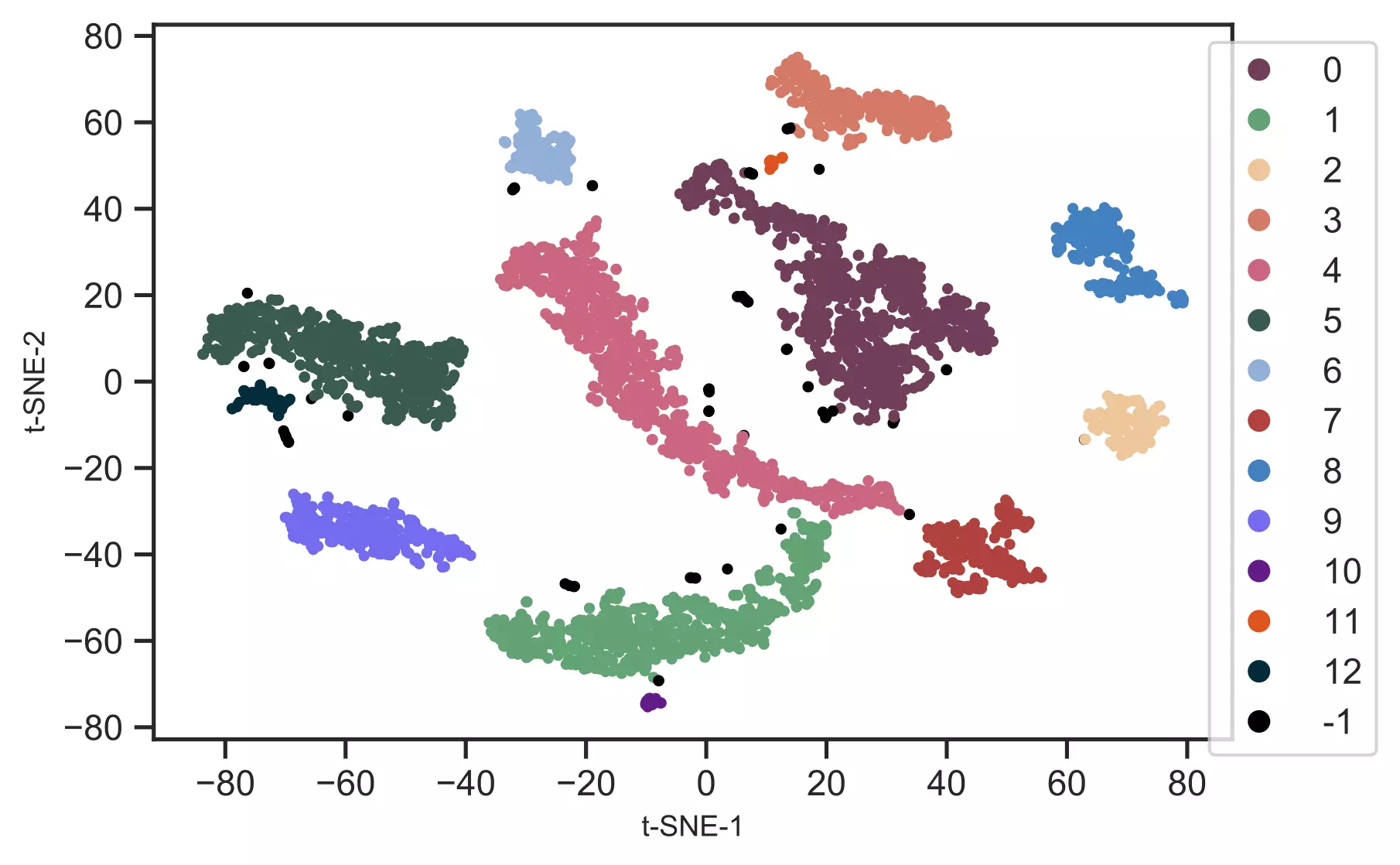
In t-SNE scatter plot, the points within the individual clusters are highly similar to each other and in distant to points in other clusters. The same pattern likely holds in a high-dimensional original dataset. In the context of scRNA-seq, these clusters represent the cells types with similar transcriptional profiles.
Advantages of t-SNE
- No assumption of linearity:t-SNE does not assume any relationship in the input features and it can be applied to both linear and non-linear datasets
- Preserves local structure: t-SNE preserves the structure of high-dimensional datasets i.e. the close points remain closer and distant points remain distant in low-dimensional space.
- Non-parametric method: t-SNE is a non-parametric machine learning method
Disadvantages of t-SNE
- t-SNE is slow: t-SNE is a computationally intensive technique and takes longer time on larger datasets. Hence, it is recommended to use the PCA method prior to t-SNE if the original datasets contain a very large number of input features. You should consider using UMAP dimension reduction method) for faster run time performance on larger datasets.
- t-SNE is a stochastic method: t-SNE is a stochastic method and produces slightly different embeddings if run multiple times. These different results could affect the numeric values on the axis but do not affect the clustering of the points. Therefore, t-SNE can be run several times to get the embeddings with the smallest Kullback–Leibler (KL) divergence.
- t-SNE does not preserve global geometry: While t-SNE is good at visualizing the well-separated clusters, most of the time it fails to preserve the global geometry of the data. Hence, t-SNE is not recommended for classification purposes.
- Hyperparameter optimization: t-SNE has various parameters to optimize to obtain well fitted model
Enhance your skills with courses on genomics and bioinformatics
- Genomic Data Science Specialization
- Biology Meets Programming: Bioinformatics for Beginners
- Python for Genomic Data Science
- Bioinformatics Specialization
- Command Line Tools for Genomic Data Science
- Introduction to Genomic Technologies
Enhance your skills with courses on machine learning
- Advanced Learning Algorithms
- Machine Learning Specialization
- Machine Learning with Python
- Machine Learning for Data Analysis
- Supervised Machine Learning: Regression and Classification
- Unsupervised Learning, Recommenders, Reinforcement Learning
- Deep Learning Specialization
- AI For Everyone
- AI in Healthcare Specialization
- Cluster Analysis in Data Mining
References
- Maaten LV, Hinton G. Visualizing data using t-SNE. Journal of machine learning research. 2008;9(Nov):2579-605.
- Kobak D, Berens P. The art of using t-SNE for single-cell transcriptomics. Nature communications. 2019 Nov 28;10(1):1-4.
- Cieslak MC, Castelfranco AM, Roncalli V, Lenz PH, Hartline DK. t-Distributed Stochastic Neighbor Embedding (t-SNE): A tool for eco-physiological transcriptomic analysis. Marine Genomics. 2019 Nov 26:100723.
- Rich-Griffin C, Stechemesser A, Finch J, Lucas E, Ott S, Schäfer P. Single-cell transcriptomics: a high-resolution avenue for plant functional genomics. Trends in plant science. 2020 Feb 1;25(2):186-97.
- Devassy BM, George S. Dimensionality reduction and visualisation of hyperspectral ink data Using t-SNE. Forensic Science International. 2020 Feb 12:110194.
- Linderman GC, Rachh M, Hoskins JG, Steinerberger S, Kluger Y. Fast interpolation-based t-SNE for improved visualization of single-cell RNA-seq data. Nature methods. 2019 Mar;16(3):243-5.
- Butler A, Hoffman P, Smibert P, Papalexi E, Satija R. Integrating single-cell transcriptomic data across different conditions, technologies, and species. Nature biotechnology. 2018 May;36(5):411-20.
- Ryu KH, Huang L, Kang HM, Schiefelbein J. Single-cell RNA sequencing resolves molecular relationships among individual plant cells. Plant physiology. 2019 Apr 1;179(4):1444-56.
- C. Kaynak (1995) Methods of Combining Multiple Classifiers and Their Applications to Handwritten Digit Recognition, MSc Thesis, Institute of Graduate Studies in Science and Engineering, Bogazici University.
This work is licensed under a Creative Commons Attribution 4.0 International License
Some of the links on this page may be affiliate links, which means we may get an affiliate commission on a valid purchase. The retailer will pay the commission at no additional cost to you.

