UMAP dimension reduction algorithm in Python (with example)

What is Uniform Manifold Approximation and Projection (UMAP)?
Uniform Manifold Approximation and Projection (UMAP) is a non-linear dimensionality reduction technique (similar to t-SNE) that is useful for the visualization of high-dimensional data (e.g. Single-cell RNA-seq data) in low-dimensional space (2-dimensions).
UMAP is generally compared to t-SNE as both are manifold learning algorithms and are used for mapping non-linear high-dimensional data into low-dimensional space.
In contrast to t-SNE, UMAP has superior run time performance, preserves more global structure of high-dimensional data, and can be applied on large datasets (e.g. datasets with >1M dimensions).
Why to use UMAP?
The majority of big data datasets contain hundreds or thousands of variables. Due to a large number of variables, it is impractical to visualize the data (even with pairwise scatter plots), so we must use dimensional reduction techniques to understand their structure and relationships.
As an example, single-cell RNA-seq (scRNA-seq) produces the expression data for thousands of genes and millions of cells in bioinformatics analysis. To understand biologically meaningful cluster structures, such high-dimensional datasets must be analyzed and visualized.
Interpreting such high-dimensional data would be impractical without transforming them into low-dimensional data. Using dimension reduction techniques such as UMAP, high-dimensional datasets can be reduced into two-dimensional space for visualization and understanding biologically meaningful clusters present in high-dimensional datasets.
How to perform UMAP in Python
In Python, UMAP analysis and visualization can be performed using the UMAP() function from umap-learn
package.
How to install UMAP?: You can install
umap-learnusing pip aspip install umap-learnor using conda asconda install -c conda-forge umap-learn
Here, I will use the example of scRNA-seq dataset for visualizing the hidden biological clusters using UMAP. I have downloaded the subset of scRNA-seq dataset of Arabidopsis thaliana root cells processed by 10x genomics Cell Ranger pipeline
This scRNA-seq dataset contains 4406 cells with ~75K sequence reads per cells. This dataset is pre-processed using Seurat R package and only used 2000 highly variable genes (variables or features) for UMAP cluster visualization.
Now, import the pre-processed scRNA-seq data as pandas DataFrame,
import pandas as pd

df = pd.read_csv("https://reneshbedre.github.io/assets/posts/gexp/ath_sc_expression.csv")
df.head(2)
# output
cells                AT1G01070  RPP1A  HTR12  AT1G01453  ADF10  PLIM2B  SBTI1.1  GL22  GPAT2  AT1G02570  BXL2  IMPA6  ...  PER72  RAB18  AT5G66440  AT5G66580  AT5G66590  AT5G66800  AT5G66815  AT5G66860  AT5G66985  IRX14H  PER73  RPL26B
AAACCTGAGACAGACC-1       0.51   1.40  -0.26      -0.28  -0.24   -0.14    -0.13 -0.07  -0.29      -0.31 -0.23   0.66  ...  -0.25   0.64       0.61      -0.55      -0.41      -0.43       2.01       3.01      -0.24   -0.18  -0.34    1.16
AAACCTGAGATCCGAG-1      -0.22   1.36  -0.26      -0.28  -0.60   -0.51    -0.13 -0.07  -0.29      -0.31  0.81  -0.31  ...  -0.25   1.25      -0.48      -0.55      -0.41      -0.43      -0.24       0.89      -0.24   -0.18  -0.49   -0.68

# set first column as index
df = df.set_index('cells')

# check the dimension (rows, columns)
df.shape
# output
(4406, 2000)
This scRNA-seq dataset consists of 4406 cells and 2000 genes. This high-dimensional data (2000 gene features) could not be visualized using a scatter plot.
Hence, we will use the UMAP() function to reduce the high-dimensional data (2000 features) to 2-dimensional data. By default,
UMAP reduces the high-dimensional data to 2-dimension.
Note: As UMAP is a stochastic algorithm, it may produce slightly different results if run multiple times. To reproduce similar results, you can use the
random_stateparameter inUMAP()function.
import umap

embedding = umap.UMAP(random_state=42).fit_transform(df.values)

embedding.shape
(4406, 2)
The resulting embedding has 2-dimensions (instead of 2000) and 4406 samples (cells). Each observation (row) of the reduced data (embedding) represents the corresponding high-dimensional data.
Now, visualize the UMAP clusters as a scatter plot,
import matplotlib.pyplot as plt

plt.scatter(embedding[:, 0], embedding[:, 1])
plt.title('UMAP clustering of 4406 cells', fontsize=20)
plt.xlabel('UMAP_1')
plt.ylabel('UMAP_2')
plt.show()
Generated UMAP cluster plot,
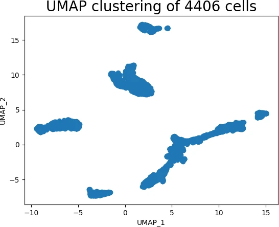
The above scatter plot suggests that the UMAP method was able to identify the structure of the high-dimensional data in low-dimensional space.
Note: UMAP has four major hyperparameters including
n_neighbors,min_dist,metric, andn_componentsthat have a signficant impact on building the effective model and clustering. Please check detailed description of how to optimize these parameters here
As UMAP is unsupervised learning method, we do not have sample target information. Hence, I will recognize the clusters using the DBSCAN clustering algorithm. This will help to color and visualize clusters of similar data points
from sklearn.cluster import DBSCAN
from collections import Counter

# here eps parameter is very important and optimizing eps is essential
# for well defined clusters. I have run DBSCAN with several eps values
# and got good clusters with eps=3
get_clusters = DBSCAN(eps = 3, min_samples = 4).fit_predict(embedding)

# check unique clusters
set(get_clusters)
# output
{0, 1, 2, 3, 4}

# get count of samples in each cluster
Counter(get_clusters)
Counter({1: 1938, 0: 1175, 2: 775, 4: 289, 3: 229})
A DBSCAN clustering algorithm predicted five clusters in the UMAP embedding dataset, which is likely representative of the cluster structure of the high-dimensional dataset. A total of 1938 samples are included in the first cluster, which is the largest.
Now, visualize the individual cluster using scatter plot,
s = plt.scatter(embedding[:, 0], embedding[:, 1], c = get_clusters, cmap = 'viridis')
plt.xlabel('UMAP_1')
plt.ylabel('UMAP_2')
plt.legend(s.legend_elements()[0], list(set(get_clusters)))
plt.title('UMAP clustering of 4406 cells', fontsize=20)
plt.show()
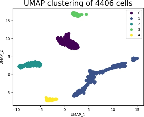
In UMAP scatter plot, the points within the individual clusters are highly similar to each other and in distant to points in other clusters. The same pattern likely holds in a high-dimensional original dataset. In the context of scRNA-seq, these clusters represent the cells types with similar transcriptional profiles and explores the transcriptomic variability among clusters.
Advantages of UMAP
- No assumption of linearity: UMAP does not assume any relationship in the input features and it can be applied to non-linear datasets
- UMAP is faster: As compared to t-SNE, UMAP has a shorter running time
- Preserves local and global structure: UMAP preserves the both local and global structure of high-dimensional data in low-dimensional space. This is an advantage over t-SNE as it fails to preserve the global structure.
- Large dataset: UMAP works efficiently on a large dataset including a high-dimensional sparse dataset. UMAP is also tested on a dataset that has > 1M dimensions.
- Distance functions: Various distance functions including metric and non-metric distance (e.g. cosine, correlation) functions
can be used with UMAP.
Disadvantages of UMAP
- UMAP is a stochastic method: UMAP is a stochastic algorithm and produces slightly different results if run multiple times. These different results could affect the numeric values on the axis but do not affect the clustering of the points.
- Hyperparameter optimization: UMAP has various hyperparameters to optimize to obtain well fitted model
Enhance your skills with courses on genomics and bioinformatics
- Genomic Data Science Specialization
- Biology Meets Programming: Bioinformatics for Beginners
- Python for Genomic Data Science
- Bioinformatics Specialization
- Command Line Tools for Genomic Data Science
- Introduction to Genomic Technologies
Enhance your skills with courses on machine learning
- Advanced Learning Algorithms
- Machine Learning Specialization
- Machine Learning with Python
- Machine Learning for Data Analysis
- Supervised Machine Learning: Regression and Classification
- Unsupervised Learning, Recommenders, Reinforcement Learning
- Deep Learning Specialization
- AI For Everyone
- AI in Healthcare Specialization
- Cluster Analysis in Data Mining
References
- McInnes, L, Healy, J, UMAP: Uniform Manifold Approximation and Projection for Dimension Reduction, ArXiv e-prints 1802.03426, 2018
- Becht E, McInnes L, Healy J, Dutertre CA, Kwok IW, Ng LG, Ginhoux F, Newell EW. Dimensionality reduction for visualizing single-cell data using UMAP. Nature biotechnology. 2019 Jan;37(1):38-44.
This work is licensed under a Creative Commons Attribution 4.0 International License
Some of the links on this page may be affiliate links, which means we may get an affiliate commission on a valid purchase. The retailer will pay the commission at no additional cost to you.

