Binary Logistic Regression in R
Binary logistic regression is used for modeling the relationship between one or more independent variables and categorical dependent variable.
In binary logistic regression, the dependent variable is binary meaning that it has two output levels (e.g. disease or healthy, 0 or 1, etc.).
In R, the binary logistic regression can be performed using the glm() function.
The general syntax of glm() for binary logistic regression looks like this:
glm(formula, family = binomial(), data = df)
The following examples explain how to perform binary logistic regression in R. We will use the subset of the breast cancer dataset (from UCI machine learning repository) to develop a prediction model using logistic regression. This model will be useful to predict whether the new patient has cancer or not based on common features.
Load the input data
This breast cancer dataset has four features (independent variables) and one binary dependent variable,
# load data
df <- read.csv("https://reneshbedre.github.io/assets/posts/logit/breast_cancer_sample.csv")

# view first few rows
head(df)
  Age      BMI Glucose Insulin diagnosis
1  48 23.50000      70   2.707         0
2  83 20.69049      92   3.115         0
3  82 23.12467      91   4.498         0
4  68 21.36752      77   3.226         0
5  86 21.11111      92   3.549         0
6  49 22.85446      92   3.226         0
The diagnosis is a binary dependent variable and indicates cancer (1) or healthy (0) patients. The Age, Glucose,
BMI, and Insulin are four independent variables.
Summarise the data
# summarise features
sapply(df[,-5], summary)

# output
             Age      BMI  Glucose  Insulin
Min.    24.00000 18.37000  60.0000  2.43200
1st Qu. 45.00000 22.97320  85.7500  4.35925
Median  56.00000 27.66242  92.0000  5.92450
Mean    57.30172 27.58211  97.7931 10.01209
3rd Qu. 71.00000 31.24144 102.0000 11.18925
Max.    89.00000 38.57876 201.0000 58.46000

# summarise categorical dependent variable
summary(as.factor(df$diagnosis))

# output
 0  1
52 64
The summary statistics for features indicate that there are no NA values in the data. If your dataset has NA values,
you should consider dropping it.
The summary statistics for the dependent variable indicate that there are 64 cancerous patients and 52 healthy patients.
Fitting logistic regression model
Now, let’s fit the model for binary logistic regression. We will use the Generalized Linear Model (glm()) with
the family parameter set to binomial.
# binary logistic regression model
fit <- glm(diagnosis ~ Age + BMI + Glucose + Insulin, family = binomial(), data = df)
summary(fit)

# output
Call:
glm(formula = diagnosis ~ Age + BMI + Glucose + Insulin, family = binomial(),
    data = df)

Deviance Residuals:
    Min       1Q   Median       3Q      Max
-2.1965  -0.9213   0.1635   0.8208   2.0410

Coefficients:
            Estimate Std. Error z value Pr(>|z|)
(Intercept) -3.65206    2.16986  -1.683  0.09236 .
Age         -0.02276    0.01439  -1.582  0.11369
BMI         -0.12402    0.04711  -2.633  0.00848 **
Glucose      0.08536    0.02270   3.760  0.00017 ***
Insulin      0.06380    0.03912   1.631  0.10293
---
Signif. codes:  0 ‘***’ 0.001 ‘**’ 0.01 ‘*’ 0.05 ‘.’ 0.1 ‘ ’ 1

(Dispersion parameter for binomial family taken to be 1)

    Null deviance: 159.57  on 115  degrees of freedom
Residual deviance: 120.80  on 111  degrees of freedom
AIC: 130.8

Number of Fisher Scoring iterations: 6

# calculate odds ratio
exp(coef(fit))

# output
(Intercept)         Age         BMI     Glucose     Insulin
 0.02593774  0.97749225  0.88335863  1.08910839  1.06587588
Binary logistic regression model interpretation:
The regression coefficients represent the change in the log-odds of the event occurring for one-unit change in predictors
assuming all other predictors are held constant. For example, for a one-unit change in Glucose, the log-odds of the patient
becoming cancerous is increases by 0.08.
The p value associated with BMI and Glucose is significant (p < 0.05) and it suggests that these predictors
have a significant impact on cancer development.
The odds ratio for Glucose and Insulin is > 1 and suggests that a one-unit increase in Glucose and Insulin
are associated with 1.08 and 1.06 increase in the odds of a patient being cancerous.
Evaluate the model (accuracy, confusion matrix, ROC, and AUC)
Let’s evaluate the fitted model performance using various metrics on a test dataset.
Load the test dataset,
# load dataset
test_df <- read.csv("https://reneshbedre.github.io/assets/posts/logit/breast_cancer_sample_test.csv")

# view first few rows
head(test_df)
  Age   BMI Glucose Insulin diagnosis
1  75 23.00      83   4.952         0
2  34 21.47      78   3.469         0
3  29 23.01      82   5.663         0
4  25 22.86      82   4.090         0
5  24 18.67      88   6.107         0
6  38 23.34      75   5.782         0
Let’s calculate the confusion matrix and accuracy of the fitted model using a test dataset. We will use the
predict() and confusionMatrix() functions.
# load package
library(caret)

# perform prediction
# type = "response" gives predicted probabilities for each observation
pred_probs <- predict(fit, test_df, type = "response")

# convert to binary prediction (0 and 1)
pred_diagn <- ifelse(pred_probs > 0.5, 1, 0)

# confusion matrix and accuracy
caret::confusionMatrix(data = as.factor(pred_diagn), reference = as.factor(test_df$diagnosis))

# output
Confusion Matrix and Statistics

          Reference
Prediction  0  1
         0 17  4
         1  6 19

               Accuracy : 0.7826
                 95% CI : (0.6364, 0.8905)
    No Information Rate : 0.5
    P-Value [Acc > NIR] : 7.821e-05

                  Kappa : 0.5652

 Mcnemar's Test P-Value : 0.7518

            Sensitivity : 0.7391
            Specificity : 0.8261
         Pos Pred Value : 0.8095
         Neg Pred Value : 0.7600
             Prevalence : 0.5000
         Detection Rate : 0.3696
   Detection Prevalence : 0.4565
      Balanced Accuracy : 0.7826

       'Positive' Class : 0
The accuracy of the binary logistic regression model is 78.26%.
In addition to accuracy, the area under the receiver operating characteristic (ROC) curve (AUC) can be used for evaluating the predictability of the model. The higher the AUC, the better is the model.
Get AUC,
# create a data frame of truth value and predicted probabilities
eval_df <- data.frame(test_df$diagnosis, pred_probs)
colnames(eval_df) <- c("truth", "pred_probs")
eval_df$truth <- as.factor(eval_df$truth)

# calculate AUC
# load package
library(yardstick)
roc_auc(eval_df, truth, pred_probs, event_level = "second")
# A tibble: 1 × 3
  .metric .estimator .estimate
  <chr>   <chr>          <dbl>
1 roc_auc binary         0.798
The AUC score is 79.80%
Now, plot the ROC curve,
# load package
library(yardstick)
library(ggplot2)
library(dplyr)

# plot ROC
roc_curve(eval_df, truth, pred_probs, event_level = "second") %>%
    ggplot(aes(x = 1 - specificity, y = sensitivity)) +
    geom_path() +
    geom_abline(lty = 3, col = "red") +
    coord_equal() +
    theme_bw()
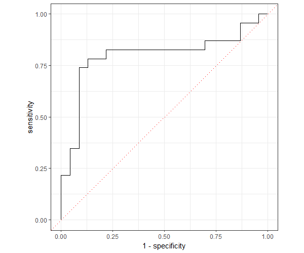
The fitted model has an AUC of 79.80% which indicates that the model has better predictability.
Related: Logistic regression in Python
Enhance your skills with courses on machine learning
- Advanced Learning Algorithms
- Machine Learning Specialization
- Machine Learning with Python
- Machine Learning for Data Analysis
- Supervised Machine Learning: Regression and Classification
- Unsupervised Learning, Recommenders, Reinforcement Learning
- Deep Learning Specialization
- AI For Everyone
- AI in Healthcare Specialization
- Cluster Analysis in Data Mining
This work is licensed under a Creative Commons Attribution 4.0 International License
Some of the links on this page may be affiliate links, which means we may get an affiliate commission on a valid purchase. The retailer will pay the commission at no additional cost to you.

