Gene expression units explained: RPM, RPKM, FPKM, TPM, DESeq, TMM, SCnorm, GeTMM, and ComBat-Seq
RNA sequencing (RNA-seq) is a state-of-the-art method for quantifying gene expression (mRNA abundance) and performing differential gene expression analysis at high resolution using Next-generation sequencing (NGS).
A number of factors influence gene quantification in RNA-seq, such as sequencing depth, gene (transcript) length, RNA composition, and sample-to-sample variability.
The gene expressions units such as CPM, RPKM, FPKM, TPM, TMM, DESeq, and so on are commonly used for quantifying the gene expression to normalize these factors.
This article provides an overview of different gene expression units, their differences, and how to calculate them from gene count data.
Why to use normalized expression units?
Normalized gene expression units provide consistent and comparable measures that can be used for performing differential expression analysis, exploratory data analysis, and comparing and visualizing gene expression counts within and across samples.
Advantages of normalized expression units,
- Normalized gene expression units are necessary to remove technical biases such as sequencing depth, RNA composition, and gene length in sequenced data. This is because more sequencing depth produces more read count for a gene expressed at the same level and differences in gene length generate unequal reads count for genes expressed at the same level (longer the gene more the read count).
- Normalized expression units make gene expressions directly comparable within and across samples.
- Normalized expression units help to remove batch effects.
Gene expression units and calculation
CPM (Counts per million)
CPM (Counts per million) is a basic gene expression unit that normalizes only for sequencing depth (depth-normalized counts). CPM is also known as RPM (Reads per million).
The CPM is biased in some applications where the gene length influences gene expression, such as RNA-seq.
CPM is calculated by dividing the mapped reads count by a per million scaling factor of total mapped reads.
CPM formula is given as,

For example, You have sequenced one library with 5 million(M) reads. Among them, total 4 M matched to the genome sequence and 5000 reads matched to a given gene.

Note: Since CPM does not consider gene length when normalizing, it is a suitable gene expression unit for sequencing protocols that generate reads regardless of gene length
You can normalize the raw read counts into CPM (or RPM) units in Python using bioinfokit
package (v0.9.1 or later). If you have not installed bioinfokit, you can install it using pip or conda.
from bioinfokit.analys import norm, get_data
# load sugarcane RNA-seq expression dataset (Published in Bedre et al., 2019)
df = get_data('sc_exp').data
df.head(2)
               gene  ctr1  ctr2  ctr3  trt1  trt2  trt3  length
0  Sobic.001G000200   338   324   246   291   202   168  1982.0
1  Sobic.001G000400    49    21    53    16    16    11  4769.0

# as this data has gene length column, we will drop length column
df = df.drop(['length'], axis=1)
# make gene column as index column
df = df.set_index('gene')
df.head(2)
                  ctr1  ctr2  ctr3  trt1  trt2  trt3
gene
Sobic.001G000200   338   324   246   291   202   168
Sobic.001G000400    49    21    53    16    16    11

# now, normalize raw counts using CPM method
nm = norm()
nm.cpm(df=df)
# get CPM normalized dataframe
cpm_df = nm.cpm_norm
cpm_df.head(2)
                        ctr1        ctr2        ctr3        trt1        trt2        trt3
gene
Sobic.001G000200  100.695004  101.731189   74.721094   92.633828   74.270713   95.314714
Sobic.001G000400   14.597796    6.593688   16.098447    5.093269    5.882829    6.240844
RPKM (Reads per kilo base of transcript per million mapped reads)
RPKM (reads per kilobase of transcript per million reads mapped) is a normalized gene expression unit that measures the gene (transcript) abundance level in a sample. RPKM is normalized to correct the gene (transcript) lengths and library sizes (sequencing depth).
RPKM is most useful for comparing gene expression values within a sample, and it is not recommended for performing differential gene expression analysis (sample-to-sample comparisons). The average RPKM values can vary from sample to sample. Generally, the higher the RPKM of a gene, the higher the expression of that gene.
RPKM calculation formula,

Here, 103 normalizes for gene length and 106 for sequencing depth factor.
FPKM (Fragments per kilo base of transcript per million mapped fragments) is a gene expression unit which is analogous to RPKM. FPKM is used especially for normalizing counts for paired-end RNA-seq data in which two (left and right) reads are sequenced from the same DNA fragment. Generally, the higher the FPKM of a gene, the higher the expression of that gene.
When we map paired-end data, both reads or only one read with high quality from a fragment can map to reference sequence. To avoid confusion or multiple counting, the fragments to which both or single read mapped are counted and represented for FPKM calculation.
RPKM calculation example,
You have sequenced one library with 5 M reads. Among them, total 4 M matched to the genome sequence and 5000 reads matched to a given gene with a length of 2000 bp.

Notes:
- RPKM considers the gene length for normalization
- RPKM is suitable for sequencing protocols where reads sequencing depends on gene length
- Used in single-end RNA-seq experiments (FPKM for paired-end RNA-seq data)
RPKM/FPKM does not represent the accurate measure of relative RNA molar concentration (rmc) and can be biased towards identifying the differentially expressed genes as the total normalized counts for each sample will be different 3,4. TPM is proposed as an alternative to the RPKM.
RPKM or FPKM normalization calculation using Pythonbioinfokit
(v0.9.1 or later) package (check how to install Python packages),
from bioinfokit.analys import norm, get_data
# load sugarcane RNA-seq expression dataset (Published in Bedre et al., 2019)
df = get_data('sc_exp').data
df.head(2)
# output
               gene  ctr1  ctr2  ctr3  trt1  trt2  trt3  length
0  Sobic.001G000200   338   324   246   291   202   168  1982.0
1  Sobic.001G000400    49    21    53    16    16    11  4769.0

# make gene column as index column
df = df.set_index('gene')
df.head(2)
# output
                  ctr1  ctr2  ctr3  trt1  trt2  trt3  length
gene
Sobic.001G000200   338   324   246   291   202   168  1982.0
Sobic.001G000400    49    21    53    16    16    11  4769.0

# now, normalize raw counts using RPKM method
# gene length must be in bp
nm = norm()
nm.rpkm(df=df, gl='length')
# get RPKM normalized dataframe
rpkm_df = nm.rpkm_norm
rpkm_df.head(2)
# output
                       ctr1       ctr2       ctr3       trt1       trt2       trt3
gene
Sobic.001G000200  50.804745  51.327542  37.699846  46.737552  37.472610  48.090169
Sobic.001G000400   3.060976   1.382614   3.375644   1.067995   1.233556   1.308627
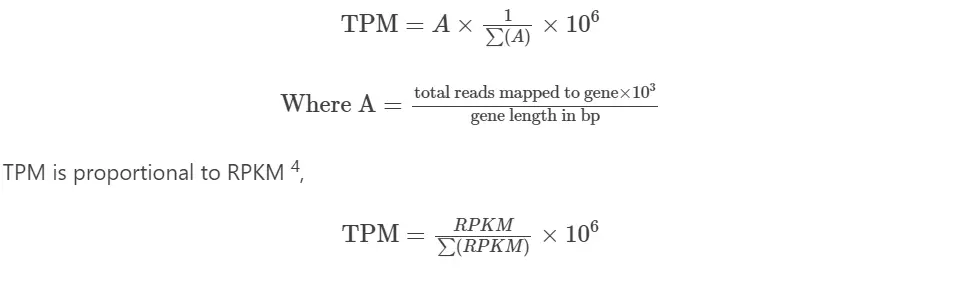
TPM (Transcripts per million)
Notes:
- TPM considers the gene length for normalization
- TPM is suitable for sequencing protocols where reads sequencing depends on gene length
TPM is proposed as an alternative to RPKM because of inaccuracy in RPKM measurement. In contrast to RPKM, the TPM average is constant and is proportional to the relative RNA molar concentration (rmc) 3,4.
TPM normalization calculation using Python bioinfokit
(v0.9.1 or later) package (check how to install Python packages),
from bioinfokit.analys import norm, get_data
# load sugarcane RNA-seq expression dataset (Published in Bedre et al., 2019)
df = get_data('sc_exp').data
df.head(2)
# output
               gene  ctr1  ctr2  ctr3  trt1  trt2  trt3  length
0  Sobic.001G000200   338   324   246   291   202   168  1982.0
1  Sobic.001G000400    49    21    53    16    16    11  4769.0

# make gene column as index column
df = df.set_index('gene')
# output
                  ctr1  ctr2  ctr3  trt1  trt2  trt3  length
gene
Sobic.001G000200   338   324   246   291   202   168  1982.0
Sobic.001G000400    49    21    53    16    16    11  4769.0

# now, normalize raw counts using TPM method
# gene length must be in bp
nm = norm()
nm.tpm(df=df, gl='length')
# get TPM normalized dataframe
tpm_df = nm.tpm_norm
tpm_df.head(2)
# output
                       ctr1       ctr2       ctr3       trt1       trt2       trt3
gene
Sobic.001G000200  99.730156  97.641941  72.361658  89.606265  69.447237  90.643338
Sobic.001G000400   6.008723   2.630189   6.479263   2.047584   2.286125   2.466582
TMM (Trimmed Mean of M-values)
- TMM is a between-sample normalization method in contrast to within-sample normalization methods (RPM, RPKM/FPKM, or TPM)
- TMM normalization method assumes that most of the genes are not differentially expressed
- TMM normalize the total RNA output among the samples and does not consider gene length or library size for normalization
- TMM considers sample RNA population and effective in normalization of samples with diverse RNA repertoires (e.g. samples from different tissues). TMM will be good choice to remove the batch effects while comparing the samples from different tissues or genotypes or in cases where RNA population would be significantly different among the samples.
- To calculate TMM,
- get the library size normalized read count for each gene in each sample
- calculate the log2 fold change between the two samples (M value)

- get absolute expression count (A value)

- Now, double trim the upper and lower percentages of the data (trim M values by 30% and A values by 5%)
- Get weighted mean of M after trimming and calculate normalization factor ( see Robinson et al., 2010 for details)
- TMM is implemented in edgeR and performs better for between-samples comparisons
- edgeR does not consider gene length for normalization as it assumes that the gene length would be constant between the samples
TMM normalization calculation using edgeR,
# load library
> library(edgeR)
> x <- read.csv("https://reneshbedre.github.io/assets/posts/gexp/df_sc.csv",row.names="gene")
# delete last column (gene length column)
> x <- x[,-7]
> head(x)
                ctr1 ctr2 ctr3 trt1 trt2 trt3
Sobic.001G000200  338  324  246  291  202  168
Sobic.001G000400   49   21   53   16   16   11
Sobic.001G000700   39   49   30   46   52   25
Sobic.001G000800  530  530  499  499  386  264
Sobic.001G001000   12    3    4    3   10    7
Sobic.001G001132    4    2    2    3    4    1

> group <- factor(c('c','c', 'c', 't', 't', 't'))
> y <- DGEList(counts=x, group=group)
# normalize for library size by cacluating scaling factor using TMM (default method)
> y <- calcNormFactors(y)
# normalization factors for each library
> y$samples
     group lib.size norm.factors
ctr1     c  3357347    1.0290290
ctr2     c  3185467    0.9918449
ctr3     c  3292872    1.0479952
trt1     t  3141934    0.9651681
trt2     t  2720231    0.9819187
trt3     t  1762881    0.9864858

# count per million read (normalized count)
> norm_counts <- cpm(y)
> head(norm_counts)
                   ctr1        ctr2        ctr3        trt1       trt2        trt3
Sobic.001G000200  97.860339 102.5561297  71.3023988  95.9799323  75.634827  96.6223700
Sobic.001G000400  14.186854   6.6471566  15.3618989   5.2772471   5.990877   6.3264647
Sobic.001G000700  11.291578  15.5100320   8.6954145  15.1720855  19.470352  14.3783289
Sobic.001G000800 153.449643 167.7615701 144.6337277 164.5841451 144.529917 151.8351528
Sobic.001G001000   3.474332   0.9495938   1.1593886   0.9894838   3.744298   4.0259321
Sobic.001G001132   1.158111   0.6330625   0.5796943   0.9894838   1.497719   0.5751332
DESeq or DESeq2 normalization (median-of-ratios method)
- The DESeq normalization method is proposed by Anders and Huber, 2010 and is similar to TMM
- DESeq normalization method also assumes that most of the genes are not differentially expressed
- The DESeq calculates size factors for each sample to compare the counts obtained from different samples with different sequencing depth
- DESeq normalization uses the median of the ratios of observed counts to calculate size factors.
- Briefly, the size factor is calculated by first dividing the observed counts for each sample by its geometric mean.
- The size factor is then calculated as the median of this ratio for each sample.
- This size factor then used for normalizing raw count data for each sample.
- DESeq or DESeq2 does not consider gene length for normalization as it assumes that the gene length would be constant between the samples.
- DESeq or DESeq2 performs better for between-samples comparisons
DESeq2 normalization calculation,
Note: DESeq2 requires raw counts (not normalized) as integer values for differential expression analysis. If you have expected counts from RSEM, it is recommended to use tximport to import the counts and then to use DESeqDataSetFromTximport() for performing differential expression analysis using DESeq2. In addition, you can also round the expected counts from RSEM but it does not offer the benefits of tximport such as normalization of transcript lengths per gene for gene-level expression analysis 13.
# load library
> library(DESeq2)
> x <- read.csv("https://reneshbedre.github.io/assets/posts/gexp/df_sc.csv",row.names="gene")
> cond <- read.csv("https://reneshbedre.github.io/assets/posts/gexp/condition.csv",row.names="sample")
> cond$condition <- factor(cond$condition)
# keep only required columns present in the sample information table
> x <- x[, rownames(cond)]
> head(x)
                 ctr1 ctr2 ctr3 trt1 trt2 trt3
Sobic.001G000200  338  324  246  291  202  168
Sobic.001G000400   49   21   53   16   16   11
Sobic.001G000700   39   49   30   46   52   25
Sobic.001G000800  530  530  499  499  386  264
Sobic.001G001000   12    3    4    3   10    7
Sobic.001G001132    4    2    2    3    4    1

# get dds
> dds <- DESeqDataSetFromMatrix(countData = x, colData = cond, design = ~ condition)
> dds <- estimateSizeFactors(dds)
# DESeq2 normalization counts
> y = counts(dds, normalized = TRUE)
> head(y)
                       ctr1       ctr2       ctr3       trt1       trt2
Sobic.001G000200 272.483741 290.412982 199.133348 272.915069 211.917896
Sobic.001G000400  39.502081  18.823064  42.902713  15.005640  16.785576
Sobic.001G000700  31.440432  43.920482  24.284555  43.141214  54.553122
Sobic.001G000800 427.267404 475.058273 403.933092 467.988384 404.952020
Sobic.001G001000   9.673979   2.689009   3.237941   2.813557  10.490985
Sobic.001G001132   3.224660   1.792673   1.618970   2.813557   4.196394
                       trt3
Sobic.001G000200 271.037655
Sobic.001G000400  17.746513
Sobic.001G000700  40.332984
Sobic.001G000800 425.916314
Sobic.001G001000  11.293236
Sobic.001G001132   1.613319

# get size factors
> sizeFactors(dds)
     ctr1      ctr2      ctr3      trt1      trt2      trt3
1.2404410 1.1156526 1.2353531 1.0662658 0.9531993 0.6198401
SCnorm for single cell RNA-seq (scRNA-seq)
- The normalization units explained above works best for bulk RNA-seq and could be biased for scRNA-seq due to abundance of zero expression counts, variable count-depth relationship (dependence of gene expression on sequencing depth), and other unwanted technical variations
- Bacher et al., 2017 proposed a SCnorm, a robust and accurate between-sample normalization unit for scRNA-seq
- Steps involved in SCnorm normalization;
- SCnorm requires the estimates of expression counts, which can be obtained from RSEM, featureCounts or HTSeq
- Genes with low expression counts are filtered out (keep the genes with atleast 10 non-zero expression counts)
- estimate the count-depth relationship using quantile regression
- Cluster genes into groups with similar count-depth relationship
- A scale factor is calculated from each group and used for estimation for normalized expression
- SCnorm is implemented in R package and is available on Bioconductor
ComBat-Seq method
- Zhang et al., 2020 proposed a ComBat-Seq (batch effect adjustment method) approach to addresses the large variance of batch effects present in RNA-seq count data
- The benefit of ComBat-Seq is that it adjusts the batch effects (technical variations in the samples such as differences in sequencing instrument for processing samples or differences in reagents or different persons performing the experiments) for raw counts data and provide the output as integer counts in contrast to other normalization methods which can produce fraction count values as described above (e.g. RPKM, TPM, TMM)
- The resulting batch adjusted integer counts can be directly used with DESeq2 which accepts only integer count data for differential gene expression analysis
- ComBat-Seq takes input as a raw un-normalized data (e.g. obtained from featureCounts or HTSeq) as input and
addresses the batch effects using a negative binomial regression model. As ComBat-Seq uses edgeR, the expected counts from RSEM can also work, but raw un-normalized counts are preferred by edgeR. - Briefly, ComBat-Seq adjust the count data by comparing the quantiles of the empirical distributions of data to the expected distribution without batch effects in the data
- ComBat-Seq is available in R
GeTMM method
- Smid et al., 2018 proposed a GeTMM (Gene length corrected TMM) which works better for both between-samples and within-sample gene expression analysis
- GeTMM is based on the TMM normalization but allows the gene length correction which lacks in TMM and DESeq or DESeq2
- In GeTMM, calculate RPK for each gene from raw read count data which is then corrected by TMM normalization factor and scaled to per million reads (See Smid et al., 2018 for detailed calculation)
GeTMM normalization using edgeR,
# load library
> library(edgeR)
> x <- read.csv("https://reneshbedre.github.io/assets/posts/gexp/df_sc.csv",row.names="gene")
# calculate reads per Kbp of gene length (corrected for gene length)
# gene length is in bp in exppression dataset and converted to Kbp
> rpk <- ( (x[,1:6]*10^3 )/x[,7])
# comparing groups
> group <- factor(c('c','c', 'c', 't', 't', 't'))
> y <- DGEList(counts=rpk, group=group)
# normalize for library size by cacluating scaling factor using TMM (default method)
> y <- calcNormFactors(y)
# normalization factors for each library
> y$samples
    group  lib.size norm.factors
ctr1     c 1709962.4    1.0768821
ctr2     c 1674190.8    0.9843634
ctr3     c 1715232.3    1.0496310
trt1     t 1638517.0    0.9841989
trt2     t 1467549.5    0.9432728
trt3     t  935125.2    0.9680985

# count per million read (normalized count)
> norm_counts <- cpm(y)
> head(norm_counts)
                      ctr1      ctr2      ctr3      trt1      trt2      trt3
Sobic.001G000200 92.610097 99.192986 68.940090 91.044874 73.623702 93.630285
Sobic.001G000400  5.579741  2.671970  6.172896  2.080457  2.423609  2.547863
Sobic.001G000700 19.324103 27.128459 15.203763 26.026360 34.273836 25.196497
Sobic.001G000800 74.410581 83.143635 71.656315 79.998205 72.089293 75.392505
Sobic.001G001000  9.283023  2.593127  3.164924  2.650027 10.290413 11.014674
Sobic.001G001132  7.464699  4.170389  3.817485  6.392849  9.929718  3.795926
Enhance your skills with courses on genomics and bioinformatics
- Genomic Data Science Specialization
- Biology Meets Programming: Bioinformatics for Beginners
- Python for Genomic Data Science
- Bioinformatics Specialization
- Command Line Tools for Genomic Data Science
- Introduction to Genomic Technologies
References
- Mortazavi A, Williams BA, McCue K, Schaeffer L, Wold B. Mapping and quantifying mammalian transcriptomes by RNA-Seq. Nature methods. 2008 Jul 1;5(7):621-8.
- Wagner GP, Kin K, Lynch VJ. Measurement of mRNA abundance using RNA-seq data: RPKM measure is inconsistent among samples. Theory in biosciences. 2012 Dec 1;131(4):281-5.
- Bullard JH, Purdom E, Hansen KD, Dudoit S. Evaluation of statistical methods for normalization and differential expression in mRNA-Seq experiments. BMC bioinformatics. 2010 Dec;11(1):94.
- Zhao S, Ye Z, Stanton R. Misuse of RPKM or TPM normalization when comparing across samples and sequencing protocols. Rna. 2020 Aug 1;26(8):903-9.
- Robinson MD, Oshlack A. A scaling normalization method for differential expression analysis of RNA-seq data. Genome biology. 2010 Mar;11(3):R25.
- Anders S, Huber W. Differential expression analysis for sequence count data. Nature Precedings. 2010 Apr 30:1-.
- Love MI, Huber W, Anders S. Moderated estimation of fold change and dispersion for RNA-seq data with DESeq2. Genome biology. 2014 Dec 1;15(12):550.
- Bacher R, Chu LF, Leng N, Gasch AP, Thomson JA, Stewart RM, Newton M, Kendziorski C. SCnorm: robust normalization of single-cell RNA-seq data. Nature methods. 2017 Jun;14(6):584.
- Zhang Y, Parmigiani G, Johnson WE. ComBat-Seq: batch effect adjustment for RNA-Seq count data. bioRxiv. 2020 Jan 1.
- Smid M, van den Braak RR, van de Werken HJ, van Riet J, van Galen A, de Weerd V, van der Vlugt-Daane M, Bril SI, Lalmahomed ZS, Kloosterman WP, Wilting SM. Gene length corrected trimmed mean of M-values (GeTMM) processing of RNA-seq data performs similarly in intersample analyses while improving intrasample comparisons. BMC bioinformatics. 2018 Dec;19(1):1-3.
- Bedre R, Irigoyen S, Schaker PD, Monteiro-Vitorello CB, Da Silva JA, Mandadi KK. Genome-wide alternative splicing landscapes modulated by biotrophic sugarcane smut pathogen. Scientific reports. 2019 Jun 20;9(1):1-2.
- Robinson MD, McCarthy DJ, Smyth GK. edgeR: a Bioconductor package for differential expression analysis of digital gene expression data. Bioinformatics. 2010 Jan 1;26(1):139-40.
- Soneson C, Love MI, Robinson MD. Differential analyses for RNA-seq: transcript-level estimates improve gene-level inferences. F1000Research. 2015;4.
If you have any questions, comments, corrections, or recommendations, please email me at reneshbe@gmail.com
This work is licensed under a Creative Commons Attribution 4.0 International License
Some of the links on this page may be affiliate links, which means we may get an affiliate commission on a valid purchase. The retailer will pay the commission at no additional cost to you.

