RNA-seq Data Analysis with DESeq2

Introduction

• Differential gene expression (DGE) analysis is commonly used in the transcriptome-wide analysis (using RNA-seq) for studying the changes in gene or transcripts expressions under different conditions (e.g. control vs infected).
• RNA sequencing (bulk and single-cell RNA-seq) using next-generation sequencing (e.g. Illumina short-read sequencing) is a de facto method for quantifying the transcriptome-wide gene or transcript expressions and performing DGE analysis.
• There are several computational tools are available for DGE analysis. In this article, I will cover DESeq2 for DGE analysis.

Check DGE analysis using edgeR

DGE analysis using DESeq2

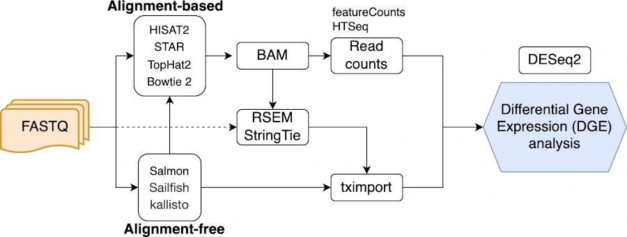
The standard workflow for DGE analysis involves the following steps

• RNA-seq with a sequencing depth of 10-30 M reads per library (at least 3 biological replicates per sample)
• aligning or mapping the quality-filtered sequenced reads to respective genome (e.g. HISAT2 or STAR). You can read my article on how to map RNA-seq reads using STAR.
• quantifying reads that are mapped to genes or transcripts (e.g. featureCounts, RSEM, HTseq)
• Raw integer read counts (un-normalized) are then used for DGE analysis using DESeq2

This standard and other workflows for DGE analysis are depicted in the following flowchart,

Note: DESeq2 requires raw integer read counts for performing accurate DGE analysis. The normalized read counts should not be used in DESeq2 analysis. DESeq2 internally normalizes the count data correcting for differences in the library sizes as sequencing depth influence the read counts (sample-specific effect). DESeq2 does not consider gene length for normalization as gene length is constant for all samples (it may not have significant effect on DGE analysis). Read more about DESeq2 normalization

Perform the DGE analysis using DESeq2 for read count matrix,

For DGE analysis, I will use the sugarcane RNA-seq data. The DGE analysis will be performed using the raw integer read counts for control and fungal treatment conditions. The goal here is to identify the differentially expressed genes under infected condition.

Note: This article focuses on DGE analysis using a count matrix. But, If you have gene quantification from Salmon, Sailfish, Kallisto, or RSEM, you can use the tximport package to import the count data to perform DGE analysis using DESeq2. Read more here

Install DESeq2 (if you have not installed before),

# R version 4.1.3 (2022-03-10) 
if (!require("BiocManager", quietly = TRUE))
    install.packages("BiocManager")

BiocManager::install("DESeq2")

Load DESeq2 and run DGE analysis,

# load library 
# DESeq2 version 1.34.0
library("DESeq2")

# get count dataset
count_matrix <- as.matrix(read.csv("https://reneshbedre.github.io/assets/posts/gexp/df_sc.csv", row.names = "gene"))
# view first two rows
head(count_matrix, 2)
                 ctr1 ctr2 ctr3 trt1 trt2 trt3 length
Sobic.001G000200  338  324  246  291  202  168   1982
Sobic.001G000400   49   21   53   16   16   11   4769

# drop length column
count_matrix <- count_matrix[, -7]
head(count_matrix, 2)
                ctr1 ctr2 ctr3 trt1 trt2 trt3
Sobic.001G000200  338  324  246  291  202  168
Sobic.001G000400   49   21   53   16   16   11

DESeq2 needs sample information (metadata) for performing DGE analysis. Let’s create the sample information (you can also import sample information if you have it in a file),

coldata <- data.frame(
   sample = c( "ctr1", "ctr2", "ctr3", "trt1", "trt2", "trt3" ),
   condition = c( "control", "control",  "control", "infected", "infected", "infected" ), 
  row.names = "sample" )
coldata$condition <- as.factor(coldata$condition)

coldata
     condition
ctr1   control
ctr2   control
ctr3   control
trt1  infected
trt2  infected
trt3  infected

Note: DESeq2 does not support the analysis without biological replicates ( 1 vs. 1 comparison). There is no other recommended alternative for performing DGE analysis without biological replicates. If you do not have any biological replicates, you can analyze log fold changes without any significance analysis.

It is essential to have the name of the columns in the count matrix in the same order as that in name of the samples (rownames in coldata). Check this article for how to reorder column names in a Data Frame.

Let’s check using the below code,

all(rownames(coldata) %in% colnames(count_matrix))
[1] TRUE

all(rownames(coldata) == colnames(count_matrix))
[1] TRUE

Now, construct DESeqDataSet for DGE analysis,

dds <- DESeqDataSetFromMatrix(countData = count_matrix, colData = coldata, 
                              design = ~ condition)

Note: The design formula specifies the experimental design to model the samples. It is used in the estimation of dispersions (spread or variability) and log2 fold changes (LFCs) of the model. The design formula also allows controlling additional factors (other than the variable of interest) in the model such as batch effects, type of sequencing, etc.

DESeq2 for paired sample: If you have paired samples (if the same subject receives two treatments e.g. before and after treatment), then you need to include the subject (sample) and treatment information in the design formula for estimating the treatment effect while considering differences in subjects. If sample and treatments are represented as subjects and condition in coldata table, then the design formula should be design = ~ subjects + condition. The factor of interest such as condition should go at the end of the formula. If you have more than two factors to consider, you should use proper multifactorial design.

Pre-filter the genes which have low counts. Low count genes may not have sufficient evidence for differential gene expression. Furthermore, removing low count genes reduce the load of multiple hypothesis testing corrections.

Here, I will remove the genes which have < 10 reads (this can vary based on research goal) in total across all the samples. Pre-filtering helps to remove genes that have very few mapped reads, reduces memory, and increases the speed of the DESeq2 analysis.

dds <- dds[rowSums(counts(dds)) >= 10,]

Now, select the reference level for condition comparisons. The reference level can set using ref parameter. The comparisons of other conditions will be compared against this reference i.e, the log2 fold changes will be calculated based on ref value (infected/control) . If this parameter is not set, comparisons will be based on alphabetical order of the levels.

# set control condition as reference
dds$condition <- relevel(dds$condition, ref = "control")

Perform differential gene expression analysis,

dds <- DESeq(dds)

# see all comparisons (here there is only one)
resultsNames(dds)
[1] "Intercept"                     "condition_infected_vs_control"

# get gene expression table
# at this step independent filtering is applied by default to remove low count genes
# independent filtering can be turned off by passing independentFiltering=FALSE to results
res <- results(dds)  # same as results(dds, name="condition_infected_vs_control") or results(dds, contrast = c("condition", "infected", "control") )
res
# output
log2 fold change (MLE): condition infected vs control 
Wald test p-value: condition infected vs control 
DataFrame with 15921 rows and 6 columns
                  baseMean log2FoldChange     lfcSE       stat     pvalue      padj
                 <numeric>      <numeric> <numeric>  <numeric>  <numeric> <numeric>
Sobic.001G000200 252.98510    -0.01225415  0.250686 -0.0488824  0.9610130  0.995253
Sobic.001G000400  25.12668    -1.04249464  0.477268 -2.1842943  0.0289406  0.280100
Sobic.001G000700  39.61157     0.48020114  0.374920  1.2808102  0.2002604  0.646876
Sobic.001G000800 434.18254    -0.00687855  0.191669 -0.0358876  0.9713720  0.997115
Sobic.001G001000   6.70029     0.61800014  0.864682  0.7147140  0.4747858  0.854971

If there are multiple group comparisons, the parameter name or contrast can be used to extract the DGE table for each comparison. Generally, contrast takes three arguments viz. column name for the condition, name of the condition for the numerator (for log2 fold change), and name of the condition for the denominator.

Order gene expression table by adjusted p value (Benjamini-Hochberg FDR method) ,

res[order(res$padj),]  
# output
log2 fold change (MLE): condition infected vs control 
Wald test p-value: condition infected vs control 
DataFrame with 15921 rows and 6 columns
                  baseMean log2FoldChange     lfcSE      stat      pvalue        padj
                 <numeric>      <numeric> <numeric> <numeric>   <numeric>   <numeric>
Sobic.003G079200   59.5931        3.99942  0.434279   9.20933 3.28163e-20 4.71570e-16
Sobic.007G191200  274.8357        3.84765  0.439166   8.76127 1.93055e-18 1.38710e-14
Sobic.004G086500   67.7705        4.15436  0.507285   8.18940 2.62539e-16 1.25756e-12
Sobic.010G095100  440.5084        1.99250  0.252985   7.87596 3.38123e-15 1.21471e-11
Sobic.004G222000   90.4653        2.60385  0.334920   7.77455 7.57139e-15 2.17602e-11

Note: You may get some genes with p value set to NA. This is due to all samples have zero counts for a gene or there is extreme outlier count for a gene or that gene is subjected to independent filtering by DESeq2.

Export differential gene expression analysis table to CSV file,

write.csv(as.data.frame(res[order(res$padj),] ), file="condition_infected_vs_control_dge.csv")

Get summary of differential gene expression with adjusted p value cut-off at 0.05,

summary(results(dds, alpha=0.05))
# output
out of 15921 with nonzero total read count
adjusted p-value < 0.05
LFC > 0 (up)       : 263, 1.7%
LFC < 0 (down)     : 150, 0.94%
outliers [1]       : 7, 0.044%
low counts [2]     : 1544, 9.7%
(mean count < 7)
[1] see 'cooksCutoff' argument of ?results
[2] see 'independentFiltering' argument of ?results

# add lfcThreshold (default 0) parameter if you want to filter genes based on log2 fold change

Get normalized counts,

normalized_counts <- counts(dds, normalized=TRUE)
head(normalized_counts)
                       ctr1       ctr2       ctr3       trt1       trt2       trt3
Sobic.001G000200 272.429944 290.406092 199.121060 272.843984 211.859879 271.249618
Sobic.001G000400  39.494282  18.822617  42.900066  15.001731  16.780980  17.760392
Sobic.001G000700  31.434224  43.919440  24.283056  43.129977  54.538187  40.364526
Sobic.001G000800 427.183048 475.047002 403.908167 467.866489 404.841154 426.249399
Sobic.001G001000   9.672069   2.688945   3.237741   2.812825  10.488113  11.302067
Sobic.001G001132   3.224023   1.792630   1.618870   2.812825   4.195245   1.614581

Learn more about DESeq2 normalization

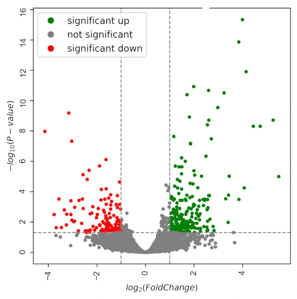
DGE Visualization

I will visualize the DGE using Volcano plot using Python,

Volcano plot,

# import packages
import pandas as pd
from bioinfokit import visuz

# import the DGE table (condition_infected_vs_control_dge.csv)
df = pd.read_csv("condition_infected_vs_control_dge.csv")
# drop NA values
df=df.dropna()

# create volcano plot
visuz.GeneExpression.volcano(df=df, lfc='log2FoldChange', pv='padj', sign_line=True, plotlegend=True)

If you want to create a heatmap, check this article

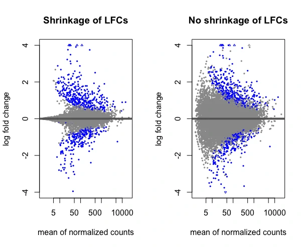
Shrinkage estimation of log2 fold changes (LFCs)

The shrinkage of effect size (LFC) helps to remove the low count genes (by shrinking towards zero). The low or highly variable read count genes can give large estimates of LFCs which may not represent true difference in changes in gene expression between two conditions.

Shrinkage estimation of LFCs can be performed on using lfcShrink and apeglm method. apeglm is a Bayesian method for shrinkage of effect sizes and gives reliable effect sizes.

resLFC <- lfcShrink(dds, coef="condition_infected_vs_control", type="apeglm")
head(resLFC)
log2 fold change (MAP): condition infected vs control 
Wald test p-value: condition infected vs control 
DataFrame with 6 rows and 5 columns
                  baseMean log2FoldChange     lfcSE    pvalue      padj
                 <numeric>      <numeric> <numeric> <numeric> <numeric>
Sobic.001G000200 252.98510    -0.00442825  0.157724 0.9610130  0.995253
Sobic.001G000400  25.12668    -0.25339744  0.407104 0.0289406  0.280100
Sobic.001G000700  39.61157     0.12383348  0.217570 0.2002604  0.646876
Sobic.001G000800 434.18254    -0.00306346  0.139306 0.9713720  0.997115
Sobic.001G001000   6.70029     0.03240858  0.201185 0.4747858  0.854971
Sobic.001G001132   2.54303     0.01295899  0.200235 0.7161400        NA

Visualize the shrinkage estimation of LFCs with MA plot and compare it without shrinkage of LFCs,

par(mfrow = c(1, 2))
plotMA(resLFC, main="Shrinkage of LFCs", ylim=c(-4,4))
plotMA(res, main="No shrinkage of LFCs", ylim=c(-4,4))

Enhance your skills with courses on genomics and bioinformatics

• Genomic Data Science Specialization
• Biology Meets Programming: Bioinformatics for Beginners
• Python for Genomic Data Science
• Bioinformatics Specialization
• Command Line Tools for Genomic Data Science
• Introduction to Genomic Technologies

References

• Love MI, Huber W, Anders S. Moderated estimation of fold change and dispersion for RNA-seq data with DESeq2. Genome biology. 2014 Dec;15(12):1-21.
• Beginner’s guide to using the DESeq2 package
• Zhu A, Ibrahim JG, Love MI. Heavy-tailed prior distributions for sequence count data: removing the noise and preserving large differences. Bioinformatics. 2019 Jun 1;35(12):2084-92.
• Stark R, Grzelak M, Hadfield J. RNA sequencing: the teenage years. Nature Reviews Genetics. 2019 Nov;20(11):631-56.

If you have any questions, comments or recommendations, please email me at reneshbe@gmail.com

This work is licensed under a Creative Commons Attribution 4.0 International License

Some of the links on this page may be affiliate links, which means we may get an affiliate commission on a valid purchase. The retailer will pay the commission at no additional cost to you.