Friedman test using Python (with examples and code)
This article explains how to perform the Friedman test in Python. You can refer to this article to know more about Friedman test, when to use Friedman test, assumptions, and how to interpret the Friedman test results.
Friedman test in Python
Friedman test data example
A researcher wants to study the effect of different locations on bacterial disease development in different plant varieties. The disease development is measured as a disease severity index with an ordinal scale (1 to 5, with 1 being no disease and 5 being severe disease symptoms). To check whether locations have an effect on disease development on each plant variety, the researcher evaluated the disease severity index for each plant variety at different locations.
Load the dataset
import pandas as pd
df=pd.read_csv("https://reneshbedre.github.io/assets/posts/anova/plant_disease_friedman.csv")
df.head(2)
`  plant_var  L1  L2  L3  L4
0        P1   4   2   5   4
1        P2   3   1   4   3

# convert to long format
df_long = pd.melt(df.reset_index(), id_vars=['plant_var'], value_vars=['L1', 'L2', 'L3', 'L4'])
df_long.columns = ['plant_var', 'locations', 'disease']
df_long.head(2)
  plant_var locations  disease
0        P1        L1        4
1        P2        L1        3
Summary statistics and visualization of dataset
Get summary statistics based on dependent variable and covariate,
from dfply import *
df_long >> group_by(X.locations) >> summarize(n=X['disease'].count(), mean=X['disease'].mean(),
                                              median=X['disease'].median(), std=X['disease'].std())
# output
  locations  n  mean  median       std
0        L1  5   4.2     4.0  0.836660
1        L2  5   1.4     1.0  0.547723
2        L3  5   4.0     4.0  0.707107
3        L4  5   4.0     4.0  0.707107
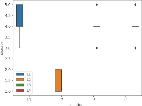
Visualize dataset,
import seaborn as sns
import matplotlib.pyplot as plt
sns.boxplot(data=df_long, x="locations", y="disease", hue=df_long.locations.tolist())
plt.show()
perform Friedman test
We will use the friedman function from pingouin package to perform Friedman test in Python
Pass the following parameters to friedman function,
- data : Dataframe (wide or long format)
- dv : Name of column in dataframe that contains dependent variable
- within : Name of column in dataframe that contains within-subject factor (treatment)
- subject : Name of column in dataframe that contains subjects (block)
import pingouin as pg

pg.friedman(data=df_long, dv="disease", within="locations", subject="plant_var")
# output
             Source         W  ddof1         Q     p-unc
Friedman  locations  0.656522      3  9.847826  0.019905
Friedman test results with chi-squared test show that there are significant differences [χ2(3) = 9.84, p = 0.01] in disease severity in plant varieties based on their locations.
Friedman test effect size
From the result above, Kendall’s W is 0.656 and indicates a large effect size (degree of difference). Kendall’s W is based on Cohen’s interpretation guidelines (0.1: small effect; 0.3: moderate effect; and >0.5: large effect).
post-hoc test
Friedman test is significant (there are significant differences among locations on disease severity), but it is an
omnibus test statistic and does not tell which locations have a significant effect on disease severity.
To know which locations are significantly different, I will perform the pairwise comparisons using the Conover post hoc test. In addition to Conover’s test, Wilcoxon-Nemenyi-McDonald-Thompson test (Nemenyi test) can also be used as post-hoc test for significant Friedman test.
The FDR method will be used to adjust the p values for multiple hypothesis testing at a 5% cut-off
I will use the posthoc_conover_friedman function from the scikit_posthocs package to perform Conover post-hoc test in
Python
Pass the following parameters to posthoc_conover_friedman function,
- a : pandas DataFrame
- y_col : Name of column in dataframe that contains dependent variable
- melted : Dataframe in long format (bool)
- group_col : Name of column in dataframe that contains within-subject factor (treatment)
- block_col : Name of column in dataframe that contains subjects (block)
- p_adjust : Adjust p value for multiple comparisons (see details here)
import scikit_posthocs as sp

sp.posthoc_conover_friedman(a=df_long, y_col="disease", group_col="locations", block_col="plant_var",
                                 p_adjust="fdr_bh", melted=True)
# output
          L1        L2        L3        L4
L1  1.000000  0.070557  0.902719  0.902719
L2  0.070557  1.000000  0.070557  0.070557
L3  0.902719  0.070557  1.000000  0.902719
L4  0.902719  0.070557  0.902719  1.000000
The multiple pairwise comparisons suggest that there are no statistically significant differences between different locations on disease severity for different plant varieties, despite there being low disease severity for location L2.
Enhance your skills with courses on Machine Learning and Python
- Machine Learning with Python
- Machine Learning for Data Analysis
- Cluster Analysis in Data Mining
- Python for Everybody Specialization
Related reading
- MANOVA using R (with examples and code)
- What is p value and how to calculate p value by hand
- Repeated Measures ANOVA using Python and R (with examples)
- ANOVA using Python (with examples)
- Multiple hypothesis testing problem in Bioinformatics
If you have any questions, comments or recommendations, please email me at reneshbe@gmail.com
This work is licensed under a Creative Commons Attribution 4.0 International License

