Calculating residuals in regression analysis [Manually and with codes]
Page content
- What is residuals?
- How to calculate residuals?
- Calculate residuals in Python
- Calculate residuals in R
What is residuals?
In regression analysis, we model the linear relationship
between one or more independent (X) variables with that of the dependent variable (y).
The simple linear regression model is given as,
\( y = a + bX + \epsilon \)
Where, a = y-intercept, b = slope of the regression line (unbiased estimate) and \( \epsilon \) = error term (residuals)
This regression model has two parts viz. fitted regression line (a + bX) and error term (ε)
The error term (ε) in regression model is called as residuals, which is difference between the actual value of y and predicted value of y (regression line).
\( residuals = actual \ y (y_i) - predicted \ y \ (\hat{y}_i) \)

How to calculate residuals?
The residual is calculated by subtracting the actual value of the data point from the predicted value of that data point. The predicted value can be obtained from regression analysis.
For example, let’s take an example of the height and weight of students (source)
| Height (X) | Weight (y) |
|---|---|
| 1.36 | 52 |
| 1.47 | 50 |
| 1.54 | 67 |
| 1.56 | 62 |
| 1.59 | 69 |
| 1.63 | 74 |
| 1.66 | 59 |
| 1.67 | 87 |
| 1.69 | 77 |
| 1.74 | 73 |
| 1.81 | 67 |
If we perform simple linear regression on this dataset, we get fitted line with the following regression equation,
ŷ = -22.4 + (55.48 * X)
Learn more here how to perform the simple linear regression in Python
With the regression equation, we can predict the weight of any student based on their height.
For example, if the height of student is 1.36, its predicted weight is 53.08
ŷ = -22.37 + (55.48 * 1.36) = 53.08
Similarly, we can calculate the predicted weight (ŷ) of all students,
Height (X) |
Weight (y) |
Predicted weight (ŷ) |
|---|---|---|
| 1.36 | 52 | 53.08 |
| 1.47 | 50 | 59.18 |
| 1.54 | 67 | 63.07 |
| 1.56 | 62 | 64.18 |
| 1.59 | 69 | 65.84 |
| 1.63 | 74 | 68.06 |
| 1.66 | 59 | 69.72 |
| 1.67 | 87 | 70.28 |
| 1.69 | 77 | 71.39 |
| 1.74 | 73 | 74.16 |
| 1.81 | 67 | 78.04 |
Now, we have actual weight (y) and predicted weight (ŷ) for calculating the residuals,
Calculate residual when height is 1.36 and weight is 52,
\( residuals = actual \ y (y_i) - predicted \ y \ (\hat{y}_i) = 52-53.08 = -1.07 \)
Similarly, we can calculate the residuals of all students,
Height (X) |
Weight (y) |
Predicted weight (y_pred) |
Residual |
|---|---|---|---|
| 1.36 | 52 | 53.08 | -1.07 |
| 1.47 | 50 | 59.18 | -9.18 |
| 1.54 | 67 | 63.07 | 3.93 |
| 1.56 | 62 | 64.18 | -2.18 |
| 1.59 | 69 | 65.84 | 3.15 |
| 1.63 | 74 | 68.06 | 5.93 |
| 1.66 | 59 | 69.72 | -10.71 |
| 1.67 | 87 | 70.28 | 16.72 |
| 1.69 | 77 | 71.39 | 5.61 |
| 1.74 | 73 | 74.16 | -1.15 |
| 1.81 | 67 | 78.05 | -11.04 |
The sum and mean of residuals is always equal to zero
If you plot the predicted data and residual, you should get residual plot as below,
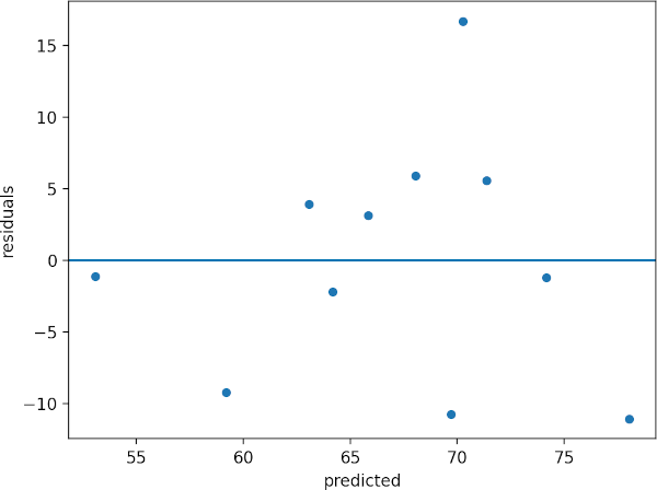
The residual plot helps to determine the relationship between X and y variables. If residuals are randomly distributed
(no pattern) around the zero line, it indicates that there linear relationship between the X and y (assumption of
linearity). If there
is a curved pattern, it means that there is no linear relationship and data is not appropriate for regression analysis.
In addition, residuals are used to assess the assumptions of normality and homogeneity of variance (homoscedasticity).
Calculate residuals in Python
Here are the steps involved in calculating residuals in regression analysis using Python,
For following steps, you need to install pandas, statsmodels, matplotlib, and seaborn Python packages. Check
how to install Python packages
Get the dataset
import pandas as pd

df = pd.read_csv("https://reneshbedre.github.io/assets/posts/reg/height.csv")
# view first two rows
df.head(2)
   Height  Weight
0    1.36      52
1    1.47      50
Fit the regression model
We will fit the simple linear regression model as there is only one independent variable
import statsmodels.api as sm

X = df['Height']  # independent variable
y = df['Weight']   # dependent variable

# to get intercept -- this is optional
X = sm.add_constant(X)

# fit the regression model
reg = sm.OLS(y, X).fit()

# to get output summary, use reg.summary()
Get the residuals
reg.resid
# output
0     -1.079016
1     -9.182056
2      3.934191
3     -2.175453
4      3.160082
5      5.940795
6    -10.723671
7     16.721507
8      5.611864
9     -1.162245
10   -11.045998
dtype: float64
Create residuals plot
Create scatterplot of predicted values and residuals,
from bioinfokit import visuz
import seaborn as sns
import matplotlib.pyplot as plt

# create a DataFrame of predicted values and residuals
df["predicted"] = reg.predict(X)
df["residuals"] = reg.resid
sns.scatterplot(data=df, x="predicted", y="residuals")
plt.axhline(y=0)
Calculate residuals in R
Here are the steps involved in calculating residuals in regression analysis using R,
Get the dataset
library(tidyverse)
df <- read.csv("https://reneshbedre.github.io/assets/posts/reg/height.csv")
# view first two rows
head(df, 2)
  Height Weight
1   1.36     52
2   1.47     50
Fit the regression model
reg <- lm(Weight ~ Height, data = df)
# to get output summary, use summary(reg)
Get the residuals
resid(reg)
         1          2          3          4          5          6          7
 -1.079016  -9.182056   3.934191  -2.175453   3.160082   5.940795 -10.723671
         8          9         10         11
 16.721507   5.611864  -1.162245 -11.045998
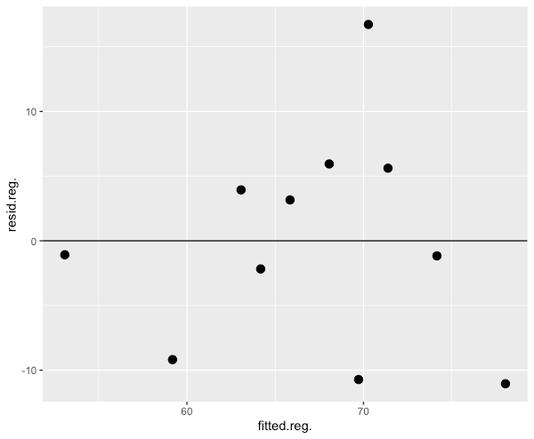
Create residuals plot
Create scatterplot of predicted values and residuals in R,
# create a data frame
df1 <- data.frame(fitted(reg), resid(reg))
ggplot(df1, aes(fitted.reg., resid.reg.)) + geom_point(size = 3) + geom_hline(yintercept = 0)
Enhance your skills with courses on regression
- Machine Learning Specialization
- Linear Regression and Modeling
- Linear Regression with Python
- Linear Regression with NumPy and Python
- Building and analyzing linear regression model in R
- Machine Learning: Regression
References
- Kim HY. Statistical notes for clinical researchers: simple linear regression 3–residual analysis. Restorative dentistry & endodontics. 2019 Feb 1;44(1).
Related reading
- Linear regression basics and implementation in Python
- Multiple linear regression (MLR)
- Mixed ANOVA using Python and R (with examples)
- Repeated Measures ANOVA using Python and R (with examples)
- ANCOVA using R (with examples and code)
- Multiple hypothesis testing problem in Bioinformatics
If you have any questions, comments or recommendations, please email me at reneshbe@gmail.com
This work is licensed under a Creative Commons Attribution 4.0 International License
Some of the links on this page may be affiliate links, which means we may get an affiliate commission on a valid purchase. The retailer will pay the commission at no additional cost to you.

