Repeated Measures ANOVA using Python and R (with examples)

Repeated measures ANOVA (Within-subjects ANOVA)

• Repeated measures ANOVA is used when the responses from the same subjects (experimental units) are measured repeatedly (more than two times) over a period of time or under different experimental conditions. For example, the number of leaves on plants measured every week for a month under certain treatment conditions.
• In repeated measure ANOVA, each subject serves as its own control, and each subject experiences all the levels of the treatments or time.
• The independent ANOVA is not appropriate for repeated measurements on the same subjects as the data violates the assumption of independence i.e. it does not interrogate within-subjects observation dependencies.
• Repeated measure ANOVA is an extension to the Paired t-test (dependent t-test) and provides similar results as of Paired t-test when there are two time points or treatments.
• Repeated measure ANOVA is mostly used in longitudinal study where subject responses are analyzed over a period of time

Assumptions of repeated measures ANOVA

• The responses from subjects (dependent variable) should be continuous
• The responses between subjects should be independent
• The subjects are randomly selected from the population
• The subject’s responses (dependent variable) should be normally distributed for each level of time or treatment (within-subjects factor). If this assumption is not met, check Friedman test for repeated measure design.
• Assumption of sphericity: the variances of differences in responses between any two levels of the independent variable (within-subjects factor) should be equal (Mauchly’s test of sphericity). This assumption also known as homogeneity-of-variance-of-differences assumption.
• There should be no outliers

Repeated measures ANOVA Hypotheses

• Null hypothesis: Treatment or time groups means are equal (no variation in means of groups)
  H₀: μ₁=μ₂=…=μ_p
• Alternative hypothesis: At least, one group mean is different from other groups
  H₁: All μ are not equal

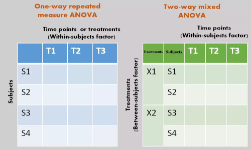
One-way repeated measures ANOVA

In one-way repeated measures ANOVA, there is only one factor (treatments or time) to study

The variation is divided into three components including variation within-subjects (SS_subjects), variation among the treatments or time points (SS_B), and residual variance (SS_E).

Source of variation	degree of freedom (Df)	Sum of squares (SS)	Mean square (MS)	F value	Significance
Subjects	Dfsubjects = n-1	SSsubjects	MSsubjects = SSsubjects ∕ Dfsubjects
Treatments or time	DfB = k-1	SSB	MSB = SSB ∕ DfB	MSB ∕ MSE	p value
Residuals or error	DfE = (n-1)(k-1)	SSE	MSE = SSE ∕ DfE
Total	DfT = nk-1	SST

Where, n = total subjects, k = level for the treatments or time

Example data ² for one-way repeated measures ANOVA analysis,

Id	W1	W2	W3	W4	W5
P1	4	5	6	8	10
P2	3	4	6	6	9
P3	6	7	9	10	12
P4	5	7	8	10	12
P5	5	6	7	8	10

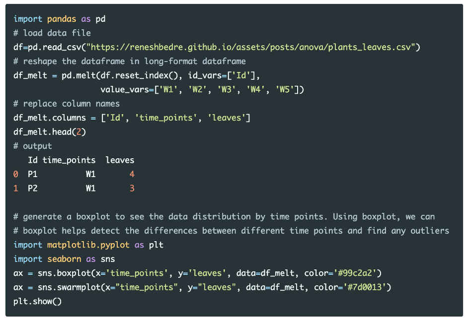
Here, there are five plants (P1 to P5) in which the number of leaves per plants were measured over multiple time points (1, 2, 3, 4 and 5 weeks) on plants at the low nutrient level. The number of leaves per plant and time points are dependent and independent variables, respectively.

Let’s perform one-way repeated measures ANOVA in Python,

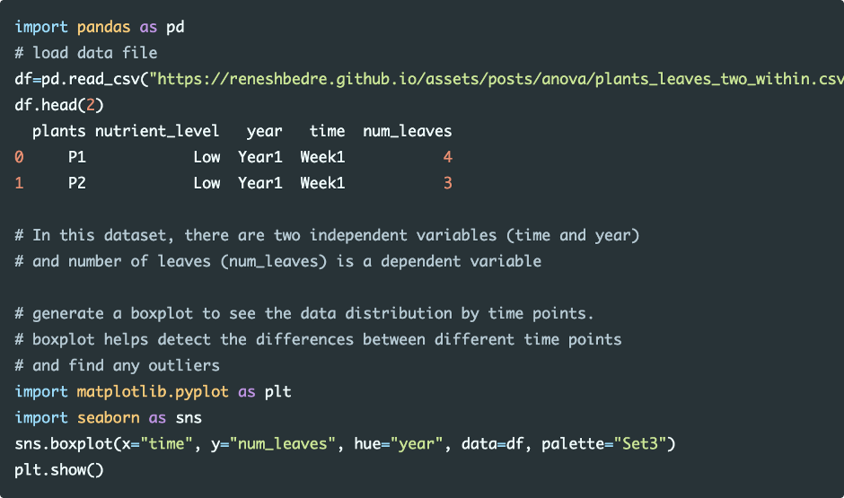
Load and visualize the dataset

Run the code in Python colab, R colab

Summary statistics

from dfply import *
df_melt >> group_by(X.time_points) >> summarize(n=X.leaves.count(), mean=X.leaves.mean(), std=X.leaves.std())

  time_points  n  mean       std
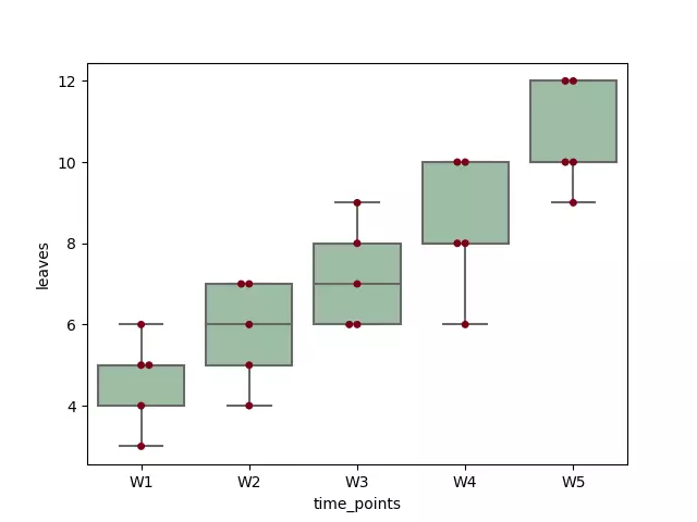
0          W1  5   4.6  1.140175
1          W2  5   5.8  1.303840
2          W3  5   7.2  1.303840
3          W4  5   8.4  1.673320
4          W5  5  10.6  1.341641

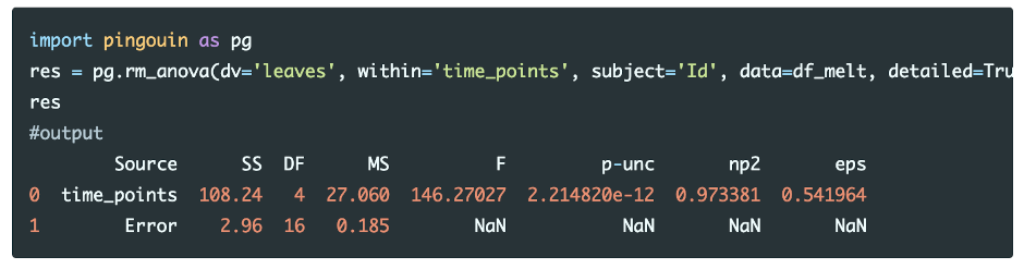
Perform one-way repeated measures ANOVA

Run the code in Python colab

From the repeated measures ANOVA results, we reject the null hypothesis in favor of the alternate hypothesis [F(4, 16) = 146.27, p <0.05, η_p²=0.97]. We conclude that the mean of the number of leaves on plants differs significantly at different time points at the low nutrient level.

The measure of effect size (Partial Eta Squared; η_p²) is 0.97 and suggests that there is a large effect of time points on a number of leaves on plants. Partial Eta Squared indicates that 97% of the overall variance (main effect and error) associated with the time points.

Note: In one-way repeated measures ANOVA, the Partial Eta Squared is the same as to Eta Squared. The reference values for effect sizes for Partial Eta Squared: small effect = 0.01; medium effect = 0.06; and large effect = 0.14

Now, we know that differences in a number of leaves on plants are statistically significant, but ANOVA output does not tell which time points are significantly different from each other. To know the pairs with significantly different time points, we will perform multiple pairwise comparison (post hoc comparison) analysis.

Post-hoc tests

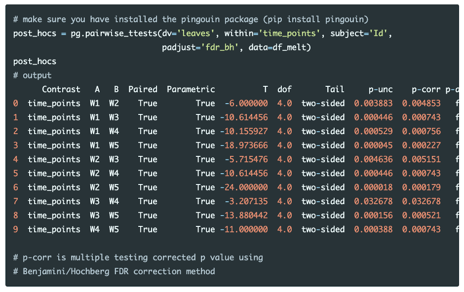
Perform multiple pairwise comparisons (t test) and corrections (Benjamini/Hochberg FDR correction),

Run the code in colab

The post-hoc tests with Benjamini/Hochberg FDR correction results indicate that all time points pairs are statistically significant (p-corr < 0.05). This concludes that the number of leaves on plants are significantly different between each time points.

Check repeated measures ANOVA assumptions

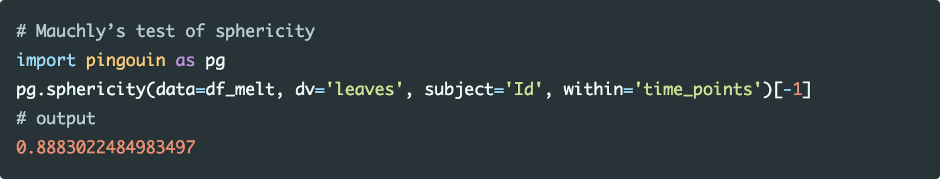
Assumption of sphericity

The assumption of sphericity can be tested using Mauchly’s test of sphericity. The violation of the assumption of sphericity can lead to an increase in type II error (loss of statistical power) and the F value is not valid.

Run the code in colab

As the p value (0.8883) is non-significant (p > 0.05), the data met the assumption of sphericity, and variances of differences of independent variables are equal.

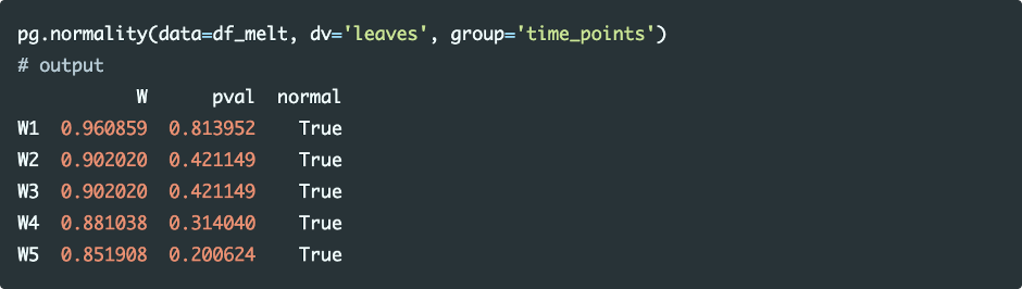
Assumption of normality

Shapiro-Wilk test can be used for checking the assumption for normality of each level of the within-subjects factor

Run the code in colab

As the p value is non-significant (p>0.05) for all levels of the within-subjects factor, we conclude that data for each time point is normally distributed.

As discussed in standard ANOVA, the visual approaches (QQ-plots and histograms) perform better than statistical tests for checking the assumption of normality.

Two-way repeated measures ANOVA (Within-within-subjects ANOVA)

In two-way repeated measures ANOVA, there are two within-subjects factors (treatments or time) to study

Let’s perform two-way repeated measures ANOVA (Within-within-subjects ANOVA) in Python,

Load and visualize the dataset

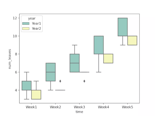
Run the code in colab

Summary statistics

from dfply import *
df >> group_by(X.year, X.time) >> summarize(n=X.num_leaves.count(), mean=X.num_leaves.mean(), std=X.num_leaves.std())

    time   year  n  mean       std
0  Week1  Year1  5   4.6  1.140175
1  Week2  Year1  5   5.8  1.303840
2  Week3  Year1  5   7.2  1.303840
3  Week4  Year1  5   8.4  1.673320
4  Week5  Year1  5  10.6  1.341641
5  Week1  Year2  5   3.6  0.894427
6  Week2  Year2  5   4.2  0.447214
7  Week3  Year2  5   5.8  0.447214
8  Week4  Year2  5   7.4  0.547723
9  Week5  Year2  5   9.6  0.547723

Perform two-way repeated measures ANOVA

import pingouin as pg
res = pg.rm_anova(dv='num_leaves', within=['time', 'year'], subject='plants', 
                  data=df, detailed=True)
res
#output
        Source      SS  ddof1  ddof2     MS           F         p-unc  p-GG-corr       np2       eps
0         time  226.88      4     16  56.72  158.657343  1.177428e-12   0.000003  0.975408  0.421229
1         year   18.00      1      4  18.00    3.600000  1.306351e-01   0.130635  0.473684  1.000000
2  time * year    0.80      4     16   0.20    1.454545  2.620704e-01   0.291675  0.266667  0.441606

Run the code in colab

From the repeated measures ANOVA results, we have two within-subjects factors (time and year; main effects) and interaction effects (time*year) to analyze.

We reject the null hypothesis in favor of the alternate hypothesis for time (F_{4, 16}=158.65, p<0.001, η_p²=0.97).

We fail to reject the null hypothesis for year (F_{1, 4}=3.6, p=0.13, η_p²=0.47), and for time and year interaction effect (F_{4, 16}=1.45, p=0.26, η_p²=0.26).

Note on F value: F value is inversely related to p value and higher F value (greater than F critical value) indicates a significant p value.

We conclude that the main effects (time) had significant effects on the number of leaves of plants at the low nutrient level.

Enhance your skills with statistical courses using R

• Statistics with R Specialization

References

1. Singh V, Rana RK, Singhal R. Analysis of repeated measurement data in the clinical trials. Journal of Ayurveda and integrative medicine. 2013 Apr;4(2):77.
2. Scheiner SM, Gurevitch J, editors. Design and analysis of ecological experiments. Oxford University Press; 2001 Apr 26.
3. Vallat, R. (2018). Pingouin: statistics in Python. Journal of Open Source Software, 3(31), 1026, https://doi.org/10.21105/joss.01026
4. Seabold, Skipper, and Josef Perktold. “statsmodels: Econometric and statistical modeling with python.” Proceedings of the 9th Python in Science Conference. 2010.
5. Schober P, Vetter TR. Repeated measures designs and analysis of longitudinal data: if at first you do not succeed—try, try again. Anesthesia and analgesia. 2018 Aug;127(2):569.
6. Maher JM, Markey JC, Ebert-May D. The other half of the story: effect size analysis in quantitative research. CBE—Life Sciences Education. 2013 Sep;12(3):345-51.

If you have any questions, comments or recommendations, please email me at reneshbe@gmail.com

This work is licensed under a Creative Commons Attribution 4.0 International License

Some of the links on this page may be affiliate links, which means we may get an affiliate commission on a valid purchase. The retailer will pay the commission at no additional cost to you.