Support Vector Machine (SVM) in Python
Support vector machine (SVM)
Introduction
- Support Vector Machine (SVM) is a supervised machine learning technique used for classification and regression tasks. SVM performs two-class or multi-class data classification by assigning the class labels to the observations.
- The goal of SVM is to map the input dataset into high-dimensional space and create a decision boundary (separating hyperplane) by learning to correctly classify the classes. (Separating) Hyperplane can be defined as the linear line in a high-dimensional space.
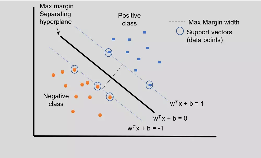
- The Hyperplane divides the input data (training data) in a such way that data points from one class will be on the same side than data points from another class, and maximize the distance between margins. Furthermore, the distance between the hyperplane and the nearest data point from each class is maximal. Hence, SVM is also known as Maximum Margin Classifiers.
- The hyperplane can be linear (linear classifier) or nonlinear (nonlinear classifier).
Linear classification using SVM
- In linear SVM, the data points from different classes can be classified by a straight line (hyperplane)
Figure 1: Linear SVM for simple two-class classification with separating hyperplane
- The soft margin SVM is useful when the training datasets are not completely linearly separable. In this case, a few misclassifications are allowed by placing the data points on the wrong side of the margin. To achieve this, the slack variable (ζi) is added to each data point.
Non-linear classification using SVM
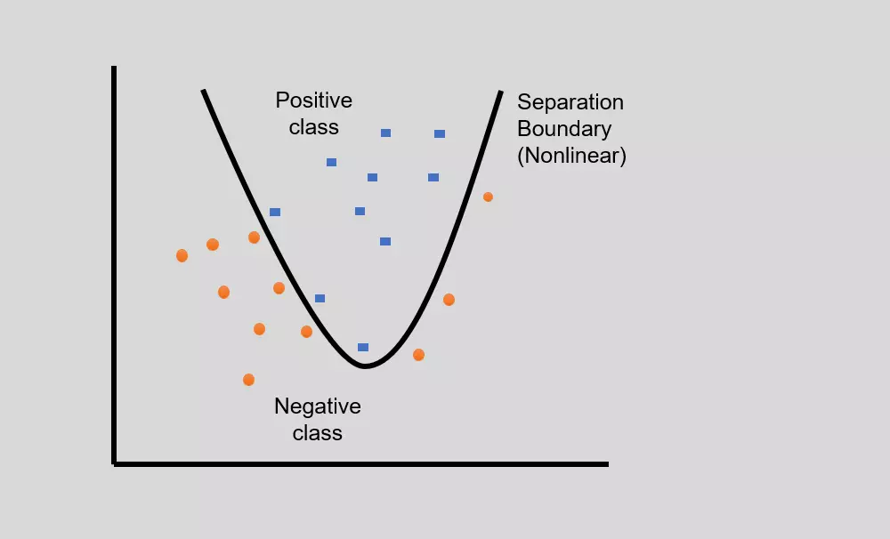
- Sometimes, in real-world problems, linear separation is not possible, and there might be curved separating hyperplane for data classification of linearly inseparable data (overlapping data).
- In such non-linear classification, the input data is mapped into high-dimensional feature space using non-linear functions (feature or kernel functions), and linear classifier is then used for data classification.
- Some well-known kernel functions include Polynomial kernel, Gaussian kernel, sigmoid kernel, Radial basis function (RBF) kernel, etc.
SVM implementation in Python
- I will use the heart disease dataset3 for patient disease classification using linear SVM.
- The heart disease dataset has 13 features, 1 class variable, and 303 data points. The class variable has two instances for classification (1: presence and 0: absence of heart disease). You can read the description of each feature here
- I will use SVM on this dataset to predict whether the patient has heart disease or not based on the 13 features (independent variables)
Load a dataset and analyze for features
import pandas as pd
# load data file
df=pd.read_csv("https://reneshbedre.github.io/assets/posts/svm/hd_cleveland.csv")
df.head(2)
# output
   age  sex  cp  rbp  chol  fbs  restecg  thalach  exang  oldpeak  slope   ca  thal  disease
0   63    1   1  145   233    1        2      150      0      2.3      3  0.0   6.0        0
1   67    1   4  160   286    0        2      108      1      1.5      2  3.0   3.0        1

# age, rbp, chol, thalach, oldpeak are continuous variables
# sex, fbs, restecg, exang, slope, ca, thal, disease are categorical variables

# make categorical variables to categorical type
cat_vars = ['sex', 'fbs', 'restecg', 'exang', 'slope', 'ca', 'thal', 'disease']
df[cat_vars] = df[cat_vars].astype('category')
Now, check and count for any missing values in the heart disease dataset (learn more how to check and handle missing values),
df.isna().sum()
# output
age        0
sex        0
cp         0
rbp        0
chol       0
fbs        0
restecg    0
thalach    0
exang      0
oldpeak    0
slope      0
ca         4
thal       2
disease    0
dtype: int64
Features ca (number of major vessels) and thal (thalassemia) are categorical variables and contains the missing
values. I will impute the missing values with the most frequent values (mode) for these features. Read more how to impute
missing values.
df['ca'].fillna(value=df['ca'].mode()[0], inplace=True)
df['thal'].fillna(value=df['thal'].mode()[0], inplace=True)

# now check if there are any missing values
df.isna().any().any()
False  # there is no any missing values
Data distribution for the outcome variable
Check the counts of the patients with heart disease (1, positive class) and without heart disease (0, negative class),
# get count plot for the heart disease outcome
from matplotlib import pyplot as plt
import seaborn as sns
ax = sns.countplot(x='disease', data=df)
plt.show()
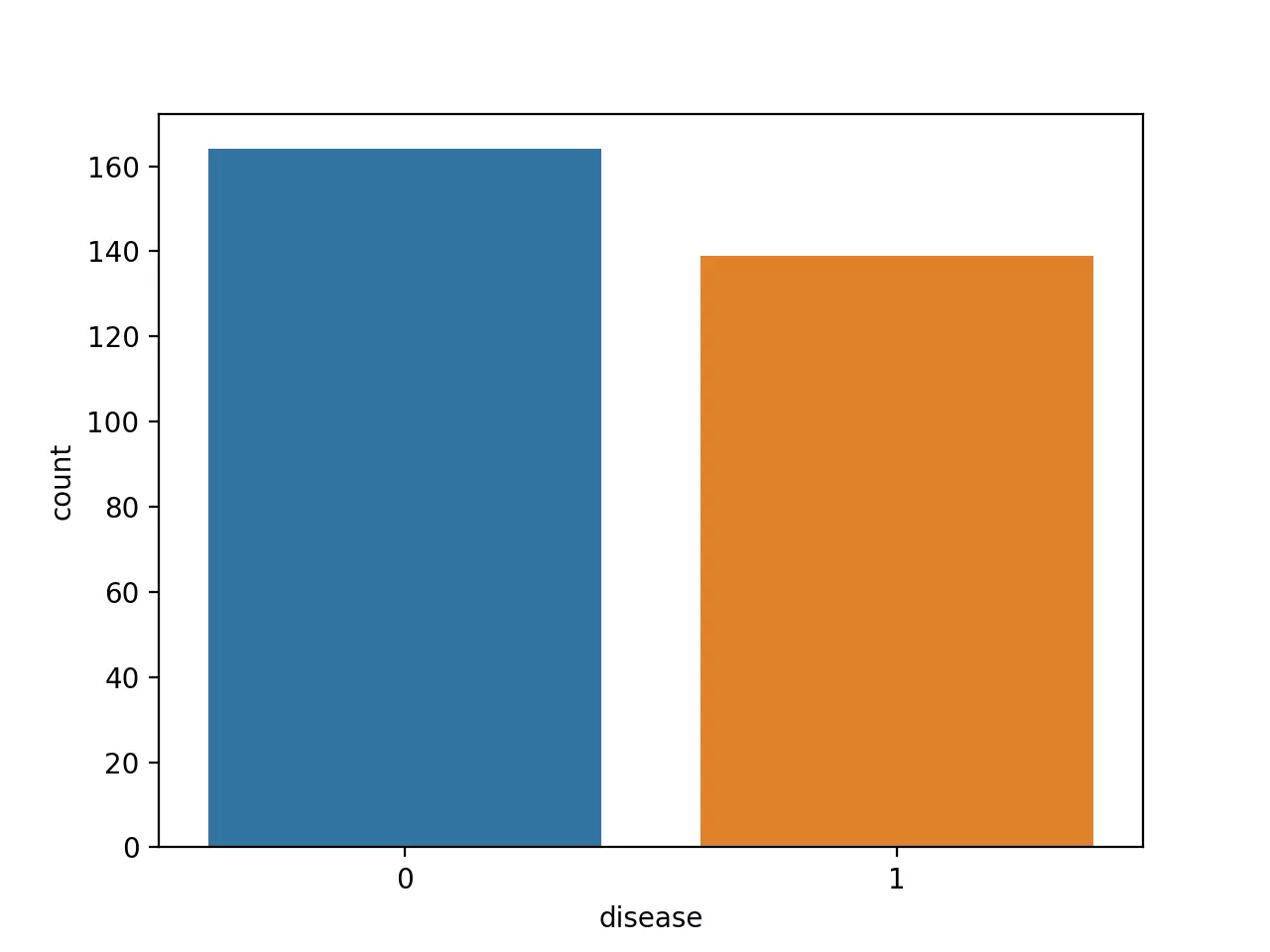
Note: It is crucial to have balanced class distribution, i.e., there should be no significant difference between positive and negative classes (commonly negative classes are more than positives in the life science field). The models trained on datasets with imbalanced class distribution tend to be biased and show poor performance toward minor class 4.
Split the dataset into training and testing datasets
Split the dataset for training (training dataset) and testing (testing dataset) for fitting the SVM model,
from sklearn.model_selection import train_test_split
# Get the independent variables
X = df.iloc[:,1:13]
# Get the dependent variables
y = df['disease']

# split the dataset into 70% as training and 30% as testing datasets
X_train, X_test, y_train, y_test = train_test_split(X, y, test_size=0.3, random_state=42)

# random_state parameter ensures that the train_test_split function will reproduce the same train and testing
# dataset every time. Set random_state to any integer.
Read my article on how to split train and test datasets in Python
Fit the SVM model with training data
Fit the SVM model using linear kernel type (linear SVM)
from sklearn.svm import SVC
svm = SVC(C=1, kernel='linear', random_state=1)
svm.fit(X=X_train, y=y_train)
Perform classification prediction using a testing dataset from fitted SVM model
y_pred = svm.predict(X=X_test)
y_pred
# output
array([1, 1, 1, 1, 1, 1, 1, 1, 0, 1, 0, 0, 1, 1, 1, 0, 0, 1, 1, 0, 0, 0,
       1, 0, 1, 0, 0, 1, 1, 1, 0, 1, 0, 0, 0, 1, 1, 0, 1, 0, 1, 0, 1, 0,
       0, 1, 0, 0, 1, 1, 0, 0, 0, 0, 1, 0, 0, 1, 1, 1, 0, 0, 0, 0, 0, 1,
       1, 0, 1, 1, 0, 0, 0, 1, 0, 1, 0, 1, 0, 1, 0, 0, 0, 0, 1, 0, 1, 0,
       1, 1, 1], dtype=int64)
Evaluate the classification prediction from the fitted SVM model
Get confusion matrix and accuracy of the classification prediction
from sklearn.metrics import classification_report, confusion_matrix, accuracy_score
# confusion matrix
confusion_matrix(y_true=y_test, y_pred=y_pred)
# output
array([[41,  7],
       [ 5, 38]], dtype=int64)

# fitted SVM model accuracy
accuracy_score(y_true=y_test, y_pred=y_pred)
# output
0.8681318681318682
Confusion matrix,
| Predicted Observed |
No heart disease (0) | Heart disease (1) |
|---|---|---|
| No heart disease (0) | 41 | 7 |
| Heart disease (1) | 5 | 38 |
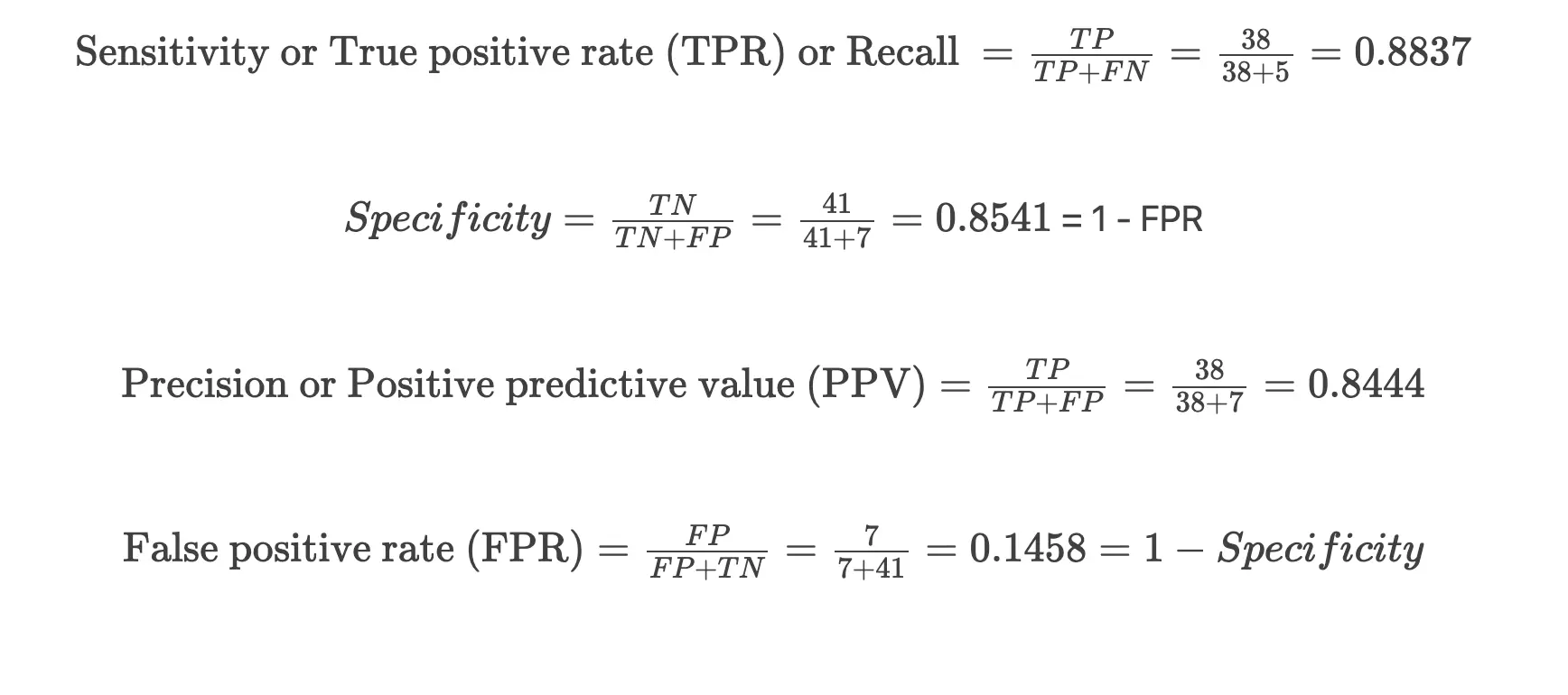
In the confusion matrix, diagonal numbers (41 and 38) indicate the correct predictions [true negative (TN) and true positives (TP)] for the absence (0) and presence (1) of heart disease outcomes for the testing dataset. The other numbers (7 and 5) indicate incorrect predictions [false positives (FP) and false negatives (FN)]
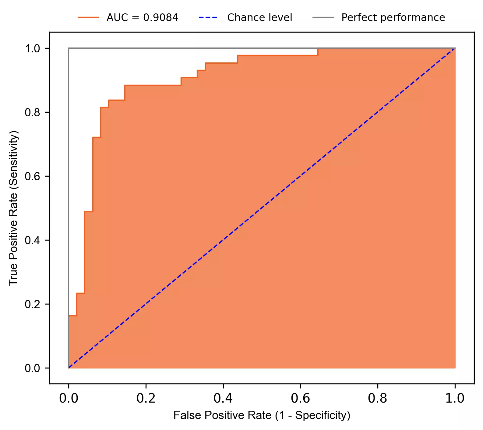
Plot Receiver Operating Characteristic (ROC) curve,
from sklearn.metrics import roc_curve, auc, roc_auc_score
from bioinfokit.visuz import stat

y_score = svm.decision_function(X=X_test)
fpr, tpr, thresholds = roc_curve(y_true=y_test, y_score=y_score)
auc = roc_auc_score(y_true=y_test, y_score=y_score)
# plot ROC
stat.roc(fpr=fpr, tpr=tpr, auc=auc, shade_auc=True, per_class=True, legendpos='upper center', legendanchor=(0.5, 1.08),
         legendcols=3)
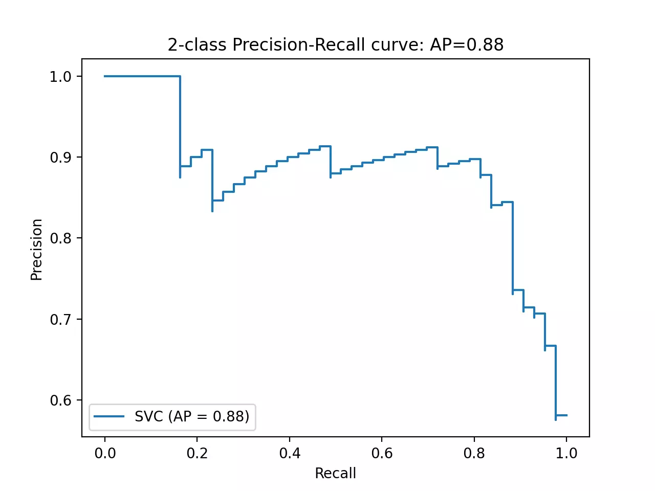
Plot area under the precision-recall curve (AUPRC),
from sklearn.metrics import precision_recall_curve, average_precision_score, plot_precision_recall_curve
import matplotlib.pyplot as plt

average_precision = average_precision_score(y_true=y_test, y_score=y_score)
# plot AUPRC
disp = plot_precision_recall_curve(estimator=svm, X=X_test, y=y_test)
disp.ax_.set_title('2-class Precision-Recall curve: '
                   'AP={0:0.2f}'.format(average_precision))
plt.show()
Conclusion
- The performance of the fitted SVM model was evaluated by area under the receiver operating characteristic curve (AUC or AUROC) and area under the precision-recall curve (AUPRC).
-
The fitted model has AUROC 0.9084 suggesting excellent predictability in classification for heart disease.
Note: AUROC can be misleading for the model trained on imbalanced datasets, and AUPRC should also be evaluated for model performance, especially when there are more negative classes. AUPRC is robust to imbalanced datasets, as it does not consider the true negatives (TN).
- The fitted model has AUPRC 0.88 (average precision) suggesting better performance. The L-shape AUPRC represents perfect classification performance.
- The accuracy of the fitted model is 0.8681. Even though accuracy is a measure of model performance, it is not alone enough. The AUC outperforms accuracy for model predictability. Two models can have the same accuracy but can differ in AUC. The models which are evaluated solely on accuracy may lead to misleading classification.
Related reading
References
- Manning CD, Raghavan P, Schütze H. Support vector machines and machine learning on documents. Introduction to Information Retrieval. 2008:319-48.
- Deka PC. Support vector machine applications in the field of hydrology: a review. Applied soft computing. 2014 Jun 1;19:372-86.
- Dua, D. and Graff, C. (2019). UCI Machine Learning Repository. Irvine, CA: University of California, School of Information and Computer Science.
- Sun Y, Wong AK, Kamel MS. Classification of imbalanced data: A review. International journal of pattern recognition and artificial intelligence. 2009 Jun;23(04):687-719.
- Mandrekar JN. Receiver operating characteristic curve in diagnostic test assessment. Journal of Thoracic Oncology. 2010 Sep 1;5(9):1315-6.
- Pedregosa F, Varoquaux G, Gramfort A, Michel V, Thirion B, Grisel O, Blondel M, Prettenhofer P, Weiss R, Dubourg V, Vanderplas J. Scikit-learn: Machine learning in Python. the Journal of machine Learning research. 2011 Nov 1;12:2825-30.
- Waskom ML. Seaborn: statistical data visualization. Journal of Open Source Software. 2021 Apr 6;6(60):3021.
If you have any questions, comments or recommendations, please email me at reneshbe@gmail.com
This work is licensed under a Creative Commons Attribution 4.0 International License

