ANCOVA using R and Python (with examples and code)
Page content
- What is ANCOVA (Analysis of Covariance)?
- Assumptions of ANCOVA
- One-way (one factor) ANCOVA in R
- post-hoc test
- Test ANCOVA assumptions
What is ANCOVA (Analysis of Covariance)?
- ANCOVA is a type of general linear model (GLM) that includes at least one continuous and one categorical independent variable (treatments). ANCOVA is useful when the effect of treatments are important while there is an additional continuous variable in the study. ANCOVA is proposed by British statistician Ronald A. Fisher during 1930s.
- The additional continuous independent variable in ANCOVA is called a covariate (also known as control, concomitant, or confounding variable).
- ANCOVA estimates the differences between groups in a categorical independent variable (primary interest) by statistically adjusting the effect of the covariate (by removing the variance associated with covariate). ANCOVA increases the statistical power and reduces error term by removing the variance associated with covariate.
- ANCOVA gives adjusted means (which are statistically controlled for covariate) for each group in a categorical independent variable. Adjusted means remove the bias of covariate from the model.
- ANCOVA uses the multiple regression approach (like simple regression in ANOVA) to study the adjusted effects of the independent variable on the dependent variable.
Assumptions of ANCOVA
ANCOVA follows similar assumptions as in ANOVA for the independence of observations, normality, and homogeneity of variances
In addition, ANCOVA needs to meet the following assumptions,
- Linearity assumption: At each level of categorical independent variable, the covariate should be linearly related to the dependent variable. If the relationship is not linear, the adjustment made to covariate will be biased.
- Homogeneity of within-group regression slopes (parallelism or non-interaction): There should be no interaction between the categorical independent variable and covariate i.e. the regression lines between the covariate and dependent variable for each group of the independent variable should be parallel (same slope).
- Dependent variable and covariate should be measured on a continuous scale
- Covariate should be measured without error or as little error as possible
One-way (one factor) ANCOVA in R
In one-way ANCOVA, there are three variables viz. one independent variable with two or more groups, dependent, and covariate variables
ANCOVA example
The following hypothetical example data consist of two independent variables viz. plant genotype (categorical) and plant genotype height (continuous). The yield of plant genotype is the dependent variable. The ANCOVA model analyze the influence of plant genotypes on genotypes yield whilst controlling the effect of covariate. With ANCOVA, the effect of different genotypes on plant yield can be precisely analyzed while controling the effect plant height.
ANCOVA Hypotheses
- Null hypothesis: Means of all genotypes yield are equal after controlling the effect of genotypes height i.e. adjusted
means are equal
H0: μ1=μ2=…=μp - Alternative hypothesis: At least, one genotype yield mean is different from other genotypes after controlling
the effect of genotypes height i.e. adjusted means are not equal
H1: All μ are not equal
Learn more about hypothesis testing and interpretation
This article explains R code for ANCOVA.
Load the dataset
library(tidyverse)
df=read_csv("https://reneshbedre.github.io/assets/posts/ancova/ancova_data.csv")
head(df, 2)
# output
  genotype height yield
  <chr>     <dbl> <dbl>
1 A          10      20
2 A          11.5    22
Summary statistics and visualization of dataset
Get summary statistics based on dependent variable and covariate,
library(rstatix)
# summary statistics for dependent variable yield
df %>% group_by(genotype) %>%  get_summary_stats(yield, type="common")
# output
  genotype variable     n   min   max median   iqr  mean    sd    se    ci
  <chr>    <chr>    <dbl> <dbl> <dbl>  <dbl> <dbl> <dbl> <dbl> <dbl> <dbl>
1 A        yield       10    20  27.5   26.5  3     25.2  2.58 0.815  1.84
2 B        yield       10    32  40     36    3.62  35.4  2.43 0.769  1.74
3 C        yield       10    15  21     17.7  2.88  17.7  2.04 0.645  1.46

# summary statistics for covariate height
df %>% group_by(genotype) %>%  get_summary_stats(height, type="common")
# output
 genotype variable     n   min   max median   iqr  mean    sd    se    ci
  <chr>    <chr>    <dbl> <dbl> <dbl>  <dbl> <dbl> <dbl> <dbl> <dbl> <dbl>
1 A        height      10    10  16.6   13.8  3.45  13.8  2.22 0.704  1.59
2 B        height      10    14  20     16.5  2.6   16.8  1.96 0.621  1.40
3 C        height      10     7  12      9.9  2.55   9.6  1.84 0.582  1.32
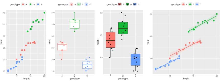
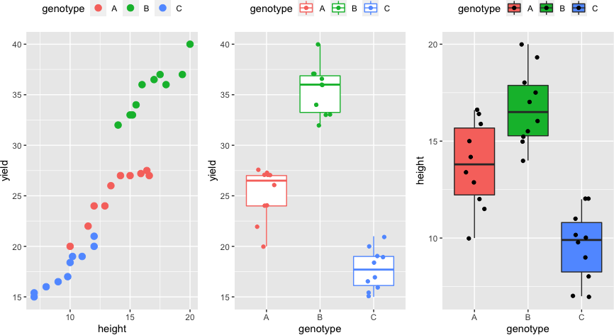
Visualize dataset,
library(gridExtra)
p1 <- ggplot(df, aes(height, yield, colour = genotype)) + geom_point(size = 3) + theme(legend.position="top")
p2 <- ggplot(df, aes(x = genotype, y = yield, col = genotype)) + geom_boxplot(outlier.shape = NA) + geom_jitter(width = 0.2) + theme(legend.position="top")
p3 <- ggplot(df, aes(x = genotype, y = height, fill = genotype)) + geom_boxplot(outlier.shape = NA) + geom_jitter(width = 0.2) + theme(legend.position="top")
grid.arrange(p1, p2, p3, ncol=3)
perform one-way ANCOVA
anova_test(data = df, formula = yield ~ height + genotype, type = 3, detailed = TRUE) # type 3 SS should be used in ANCOVA
# output
ANOVA Table (type III tests)

       Effect     SSn    SSd DFn DFd       F        p p<.05   ges
1 (Intercept)  78.071 17.771   1  26 114.220 5.22e-11     * 0.815
2      height 132.696 17.771   1  26 194.138 1.43e-13     * 0.882
3    genotype 193.232 17.771   2  26 141.353 1.07e-14     * 0.916
ANCOVA results indicate that there are significant differences in mean yield [F(2, 26) = 141.35, p < 0.001] among genotypes whilst adjusting the effect of genotype height.
The covariate height is significant [F(1, 26) = 194.13, p < 0.001] suggesting it is an important predictor of genotypes yield.
Get adjusted means,
adj_means <- emmeans_test(data = df, formula = yield ~ genotype, covariate = height)
get_emmeans(adj_means)
# output
 height genotype emmean    se    df conf.low conf.high method
   <dbl> <fct>     <dbl> <dbl> <dbl>    <dbl>     <dbl> <chr>
1   13.4 A          24.7 0.263    26     24.2      25.3 Emmeans test
2   13.4 B          31.7 0.373    26     31.0      32.5 Emmeans test
3   13.4 C          21.9 0.397    26     21.1      22.7 Emmeans test
emmeans gives the estimated marginal means (EMMs) which is also known as least-squares means. EMMs are adjusted means
for each genotype. The B genotype has the highest yield (31.7) whilst controlling the effect of height.
post-hoc test
From ANCOVA, we know that genotypes yield are statistically significant whilst controlling the effect of height, but ANCOVA does not tell which genotypes are significantly different from each other.
To know the genotypes with statistically significant differences, I will perform the post-hoc test with the Benjamini-Hochberg FDR method for multiple hypothesis testing at a 5% cut-off
emmeans_test(data = df, formula = yield ~ genotype, covariate = height, p.adjust.method = "fdr")
# output
  term  .y.   group1 group2    df statistic        p    p.adj
* <chr> <chr> <chr>  <chr>  <dbl>     <dbl>    <dbl>    <dbl>
1 heig… yield A      B         26    -16.0  5.32e-15 1.60e-14
2 heig… yield A      C         26      5.71 5.21e- 6 5.21e- 6
3 heig… yield B      C         26     14.6  4.89e-14 7.33e-14
The multiple pairwise comparisons suggest that there are statistically significant differences in adjusted yield means among all genotypes.
Test ANCOVA assumptions
Assumptions of normality
The residuals should be approximately normally distributed. The Shapiro-Wilk test can be used to check the normal distribution of residuals. Null hypothesis: data is drawn from a normal distribution.
shapiro.test(resid(aov(yield ~ genotype + height, data = df)))
# output
	Shapiro-Wilk normality test

data:  resid(aov(yield ~ genotype + height, data = df))
W = 0.96116, p-value = 0.3315
As the p value is non-significant (p > 0.05), we fail to reject the null hypothesis and conclude that data is drawn from a normal distribution.
If the sample size is sufficiently large (n > 30), the moderate departure from normality can be allowed.
In addition, QQ plot and histograms can be used to assess the assumptions of normality
Assumptions of homogeneity of variances
The variance should be similar for all genotypes. Bartlett's test can be used to check the
homogeneity of variances. Null hypothesis: samples from populations
have equal variances.
bartlett.test(yield ~ genotype, data = df)
# output
	Bartlett test of homogeneity of variances

data:  yield by genotype
Bartlett's K-squared = 0.48952, df = 2, p-value = 0.7829
As the p value is non-significant (p > 0.05), we fail to reject the null hypothesis and conclude that genotypes have equal variances.
Levene’s test can be used to check the homogeneity of variances when the data is not drawn from a normal distribution.
Assumptions of homogeneity of regression slopes (covariate coefficients)
This is important assumption in ANCOVA. There should be no interaction between the categorical independent variable and covariate. This can be tested using interaction terms between genotype and height in ANOVA. If this assumption is violated, the treatment effect will not be same across various levels of the covariate. At this stage, consider alternative to ANCOVA such as Johnson-Neyman Technique.
Anova(aov(yield ~ genotype * height, data = df), type = 3)
# output
                Sum Sq Df F value    Pr(>F)
(Intercept)     24.140  1 32.8418 6.629e-06 ***
genotype         6.756  2  4.5960   0.02042 *
height          52.014  1 70.7635 1.283e-08 ***
genotype:height  0.130  2  0.0887   0.91545
Residuals       17.641 24
As the p value is for interaction (genotype:height) is non-significant (p > 0.05), there is no interaction between genotype and height.
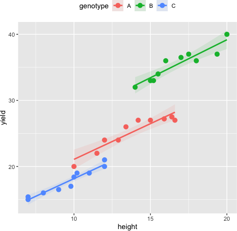
Assumptions of linearity
The relationship between the covariate and at each group of the independent variable should be linear. The scatterplot of covariate and dependent variable at each group of the independent variable can be used to assess this assumption. The data points should lie on the straight line to meet the linearity assumption.
ggplot(df, aes(height, yield, colour = genotype)) + geom_point(size = 3) +
    geom_smooth(method = "lm", aes(fill = genotype), alpha = 0.1) + theme(legend.position="top")
Enhance your skills with statistical courses using R
- ANOVA and Experimental Design
- Statistics with R Specialization
- Data Science: Foundations using R Specialization
Related reading
- MANOVA using R (with examples and code)
- Mixed ANOVA using Python and R (with examples)
- Repeated Measures ANOVA using Python and R (with examples)
- ANOVA using Python (with examples)
- Multiple hypothesis testing problem in Bioinformatics
References
- Kim HY. Statistical notes for clinical researchers: analysis of covariance (ANCOVA). Restorative dentistry & endodontics. 2018 Aug 22;43(4).
- Analysis of Covariance (ANCOVA)
- Khammar A, Yarahmadi M, Madadizadeh F. What is analysis of covariance (ANCOVA) and how to correctly report its results in medical research?. Iran J Public Health. 2018 Dec 19.
- Leppink J. Analysis of covariance (ANCOVA) vs. moderated regression (MODREG): Why the interaction matters. Health
Professions Education. 2018 Sep 1;4(3):225-32. - Sharma S. ANOVA and ANCOVA. SAGE Publications Limited; 2020.
If you have any questions, comments or recommendations, please email me at reneshbe@gmail.com
This work is licensed under a Creative Commons Attribution 4.0 International License
Some of the links on this page may be affiliate links, which means we may get an affiliate commission on a valid purchase. The retailer will pay the commission at no additional cost to you.

