DBSCAN clustering algorithm in Python (with example dataset)

What is DBSCAN?

Density Based Spatial Clustering of Applications with Noise (abbreviated as DBSCAN) is a density-based unsupervised clustering algorithm. In DBSCAN, clusters are formed from dense regions and separated by regions of no or low densities.

DBSCAN computes nearest neighbor graphs and creates arbitrary-shaped clusters in datasets (which may contain noise or outliers) as opposed to k-means clustering, which typically generates spherical-shaped clusters

Unlike k-means clustering, DBSCAN does not require specifying the number of clusters initially. However, DBSCAN requires two parameters viz. the radius of neighborhoods for a given data point p (eps or ε) and the minimum number of data points in a given ε-neighborhood to form clusters (minPts).

DBSCAN is also useful for clustering non-linear datasets.

DBSCAN common terminologies

Here we will discuss the core point, border point, noise point (Outlier), and density reachable terminologies used in DBSCAN.

The randomly selected data point p is called a core point if there are more than a minimum number of points (minPts) within a ε-neighborhood of p.

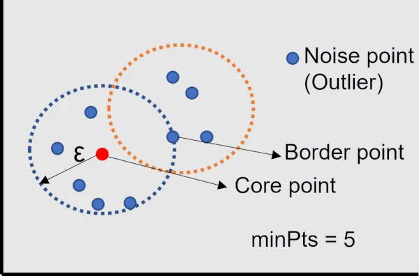
A data point is called a border point if it is within a ε-neighborhood of p and it has fewer than the minimum number of points (minPts) within its ε-neighborhood.

If a point that is not a core point or border point is called a Noise point (Outlier).

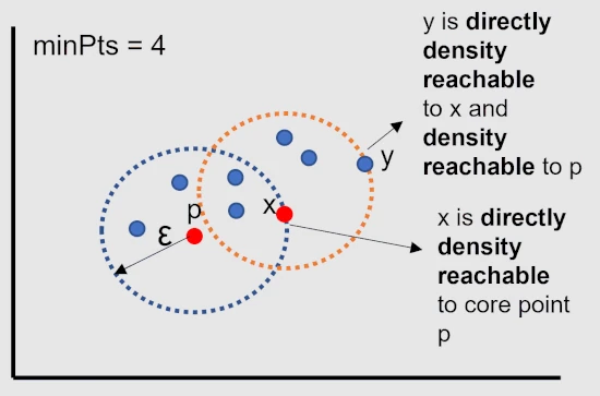
A point x is directly density reachable from point p if a point p is a core point and x is in p’s ε-neighborhood. A point y is density reachable from point p if a point y is directly density reachable to core point x, which is also density reachable to core point p.

All points within a ε-neighborhood of a core point belongs to same clusters and all points in a cluster are directly density reachable to core point.

The points which are not density reachable from any core points are called noise (outliers) points.

Steps involved in DBSCAN clustering algorithm

1. Choose any point p randomly
2. Identify all density reachable points from p with ε and minPts parameter
3. If p is a core point, create a cluster (with ε and minPts)
4. If p is a border point, visit the next point in a dataset
5. Continue the algorithm until all points are visited

Perform DBSCAN clustering in Python

To perform DBSCAN clustering in Python, you will require to install sklearn, pandas, and matplotlib Python packages. Check for how to install Python packages

Get dataset

For clustering using DBSCAN, I am using a single-cell gene expression dataset of Arabidopsis thaliana root cells processed by a 10x genomics Cell Ranger pipeline. The dataset is preprocessed t-SNE dimensionality reduction technique. Now, I will use the t-SNE embedding vectors to identify the clusters using DBSCAN.

import pandas as pd

df = pd.read_csv("https://reneshbedre.github.io/assets/posts/tsne/tsne_scores.csv")
df.head(2)
     t-SNE-1    t-SNE-2
0  10.846841 -16.712580
1  24.794334 -16.775398

# check the shape of dataset
print(df.shape)
(4406, 2)

This dataset has 4406 rows and two features. This is unlabelled dataset (no cluster information). I will identify the cluster information on this dataset using DBSCAN.

Compute required parameters for DBSCAN clustering

DBSCAN requires ε and minPts parameters for clustering. The minPts parameter is easy to set. The minPts should be 4 for two-dimensional dataset. For multidimensional dataset, minPts should be 2 * number of dimensions. For example, if your dataset has 6 features, set minPts = 12. Sometimes, domain expertise is also required to set a minPts parameter.

Another question is what optimal value should be used for the ε parameter. The ε parameter is difficult to set and depends on the distance function. Sometimes, domain expertise is also required to set a ε parameter. The ε should be as small as possible.

To determine the optimal ε parameter, I will compute the k-nearest neighbor (kNN) distances (average distance of every data point to its k-nearest neighbors) of an input dataset using the k-nearest neighbor method (unsupervised nearest neighbors learning). For finding the k-nearest neighbor, I will use the sklearn.neighbors.NearestNeighbors function.

NearestNeighbors function requires n_neighbors (number of neighbors) parameter, which can be same as the minPts value.

import numpy as np
from sklearn.neighbors import NearestNeighbors
# n_neighbors = 5 as kneighbors function returns distance of point to itself (i.e. first column will be zeros) 
nbrs = NearestNeighbors(n_neighbors = 5).fit(df)
# Find the k-neighbors of a point
neigh_dist, neigh_ind = nbrs.kneighbors(df)
# sort the neighbor distances (lengths to points) in ascending order
# axis = 0 represents sort along first axis i.e. sort along row
sort_neigh_dist = np.sort(neigh_dist, axis = 0)

Now, get the sorted k^th column (distances with k^th neighbors) and plot the kNN distance plot,

import matplotlib.pyplot as plt
k_dist = sort_neigh_dist[:, 4]
plt.plot(k_dist)
plt.ylabel("k-NN distance")
plt.xlabel("Sorted observations (4th NN)")
plt.show()

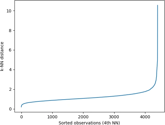
In the k-NN distance plot, you should look for the “knee” or “elbow” point (a threshold value where you see a sharp change) of the curve to find the optimal value of ε.

Identifying the exact knee point could be difficult visually. In the below plot, the knee point can occur at any point between 2 to 5 i.e. the points below knee point belong to a cluster, and points above the knee point are noise or outliers (noise points will have higher kNN distance). You should run DBSCAN based on different values of ε (between 2 and 5) to find the best ε that gives the best clustering.

Additionally, to get an estimate of knee point, you can use the KneeLocator() function from the kneed package.

from kneed import KneeLocator
kneedle = KneeLocator(x = range(1, len(neigh_dist)+1), y = k_dist, S = 1.0, 
                      curve = "concave", direction = "increasing", online=True)

# get the estimate of knee point
print(kneedle.knee_y)
4.5445133515748894

Distance plot,

kneedle.plot_knee()
plt.show()

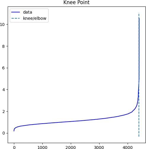
We will use 4.54 as optimum value of ε for DBSCAN clustering

Compute DBSCAN clustering

Now, we have calculated ε and minPts parameters for DBSCAN clustering. We will pass these parameters to the DBSCAN to predict the clusters using the sklearn.cluster.DBSCAN class.

from sklearn.cluster import DBSCAN
clusters = DBSCAN(eps = 4.54, min_samples = 4).fit(df)
# get cluster labels
clusters.labels_
# output
array([0, 0, 1, ..., 1, 1, 1], dtype=int64)

# check unique clusters
set(clusters.labels_)
{0, 1, 2, 3, 4, 5, 6, 7, 8, 9, 10, -1}
# -1 value represents noisy points could not assigned to any cluster

Choosing appropriate DBSCAN parameters can be harder sometimes. If you select ε based on your domain expertise, you should play with different values of minPts to get better insights from clustering.

Get each cluster size,

from collections import Counter
Counter(clusters.labels_)
# output
Counter({1: 1524, 0: 870, 2: 769, 3: 301, 7: 283, 5: 246, 6: 232, 4: 153, 8: 11, 10: 8, 9: 6, -1: 3})

DBSCAN clustering identified 11 clusters with given parameters. The largest cluster (1) has 1524 data points and the smallest cluster (9) has 6 data points.

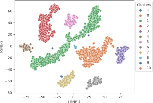
Visualization of DBSCAN clustering

Visualize the cluster as a scatter plot and color the clusters using predicted class labels,

import seaborn as sns
import matplotlib.pyplot as plt
p = sns.scatterplot(data = df, x = "t-SNE-1", y = "t-SNE-2", hue = clusters.labels_, legend = "full", palette = "deep")
sns.move_legend(p, "upper right", bbox_to_anchor = (1.17, 1.), title = 'Clusters')
plt.show()

Different colors represent different predicted clusters. Blue represents noisy points (-1 cluster).

DBSCAN limitations

• DBSCAN is computationally expensive (less scalable) and more complicated clustering method as compared to simple k-means clustering
• DBSCAN is sensitive to input parameters, and it is hard to set accurate input parameters
• DBSCAN depends on a single value of ε for all clusters, and therefore, clusters with variable densities may not be correctly identified by DBSCAN
• DBSCAN is a time-consuming algorithm for clustering

Enhance your skills with courses on machine learning

• Advanced Learning Algorithms
• Machine Learning Specialization
• Machine Learning with Python
• Machine Learning for Data Analysis
• Supervised Machine Learning: Regression and Classification
• Unsupervised Learning, Recommenders, Reinforcement Learning
• Deep Learning Specialization
• AI For Everyone
• AI in Healthcare Specialization
• Cluster Analysis in Data Mining

Related reading

• Performing and visualizing the Principal component analysis (PCA) from PCA function and scratch in Python
• Support Vector Machine (SVM) basics and implementation in Python
• Logistic regression in Python (feature selection, model fitting, and prediction)
• k-means clustering in Python [with example]

References

• Chen Y, Ruys W, Biros G. KNN-DBSCAN: a DBSCAN in high dimensions. arXiv preprint arXiv:2009.04552. 2020 Sep 9.
• Ryu KH, Huang L, Kang HM, Schiefelbein J. Single-cell RNA sequencing resolves molecular relationships among individual plant cells. Plant physiology. 2019 Apr 1;179(4):1444-56.
• Dudik JM, Kurosu A, Coyle JL, Sejdić E. A comparative analysis of DBSCAN, K-means, and quadratic variation algorithms for automatic identification of swallows from swallowing accelerometry signals. Computers in biology and medicine. 2015 Apr 1;59:10-8.
• Ester M, Kriegel HP, Sander J, Xu X. A density-based algorithm for discovering clusters in large spatial databases with noise. Inkdd 1996 Aug 2 (Vol. 96, No. 34, pp. 226-231).
• Xie X, Duan L, Qiu T, Li J. Quantum algorithm for MMNG-based DBSCAN. Scientific Reports. 2021 Jul 30;11(1):1-8.
• Schubert E, Sander J, Ester M, Kriegel HP, Xu X. DBSCAN revisited, revisited: why and how you should (still) use DBSCAN. ACM Transactions on Database Systems (TODS). 2017 Jul 31;42(3):1-21.

If you have any questions, comments, corrections, or recommendations, please email me at reneshbe@gmail.com

Subscribe to get new article to your email when published

* indicates required

Email Address *

This work is licensed under a Creative Commons Attribution 4.0 International License

Some of the links on this page may be affiliate links, which means we may get an affiliate commission on a valid purchase. The retailer will pay the commission at no additional cost to you.