8 methods to find outliers in R (with examples)
Page content
What is an outlier?
Outlier is an unusual observation that is not consistent with the remaining observations in a sample dataset.
The outliers in a dataset can come from the following possible sources,
- contaminated data samples
- data points from different population
- incorrect sampling methods,
- underlying significant treatment response (e.g. biological variation of samples),
- error in data collection or analysis.
Why to find outliers in a dataset?
Outliers can largely influence the results of the statistical tests and hence it is necessary to find the outliers in the dataset.
Most of the statistical tests and machine learning methods are sensitive to outliers and they must be removed before performing the analysis.
For example,
- the presence of outliers can affect the normal distribution of the dataset which is a basic assumption in most of parametric hypothesis-based tests
- the presence of outlier distort the mean and standard deviation of the dataset
- In k-means clustering, the presence of outliers can significantly affect the clustering and may not give well-separated cluster.
Statistical methods to find outliers
Histogram, scatter plot, and boxplot
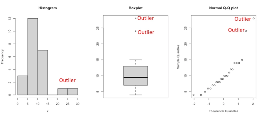
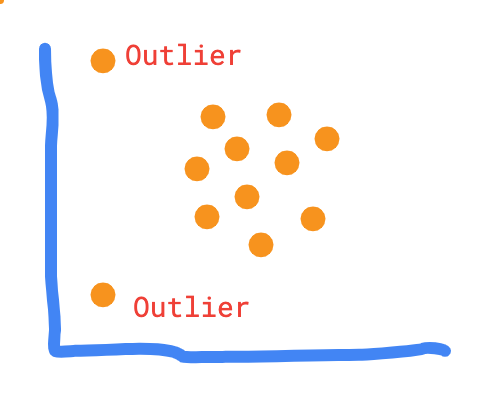
Visual approaches such as histogram, scatter plot (such as Q-Q plot), and boxplot are the easiest method to detect outliers.
Let’s take an example of this univariate dataset [10,4,6,8,9,8,7,6,12,14,11,9,8,4,5,10,14,12,15,7,10,14,24,28] and identify outliers using visual approaches (all of the R code mentioned in this article are implemented in RStudio),
# RStudio console
library(gridExtra)
x = c(10,4,6,8,9,8,7,6,12,14,11,9,8,4,5,10,14,12,15,7,10,14,24,28)
# histogram, Q-Q plot, and boxplot
par(mfrow = c(1, 3))
hist(x, main = "Histogram")
boxplot(x, main = "Boxplot")
qqnorm(x, main = "Normal Q-Q plot")
Mean and Standard deviation (SD)
The Standard deviation (SD) and mean of the data can be used for finding the outliers in the dataset. The minimum (Tmin) and maximum (Tmax) threshold based on mean and SD for identifying outliers is given as,

Where α is the threshold factor for defining the number of SD. Generally, the data point which is 3 (α = 3) SD away from the mean is considered as an outlier.
This method works well if the data is normally distributed and when there are very less percentages of outliers in the dataset. It is also sensitive to outliers as mean and SD will change if the outlier is present.
Calculate Mean and Standard deviation (SD) in R,
x = c(10,4,6,8,9,8,7,6,12,14,11,9,8,4,5,10,14,12,15,7,10,14,24,28)

# get mean and Standard deviation
mean = mean(x)
std = sd(x)

# get threshold values for outliers
Tmin = mean-(3*std)
Tmax = mean+(3*std)

# find outlier
x[which(x < Tmin | x > Tmax)]
[1] 28

# remove outlier
x[which(x > Tmin & x < Tmax)]
 [1] 10  4  6  8  9  8  7  6 12 14 11  9  8  4  5 10 14 12 15  7 10 14 24
The mean and Standard deviation (SD) method identified the value 28 as an outlier.
The other variant of the SD method is to use the Clever Standard deviation (Clever SD) method, which is an iterative process to remove outliers. In each iteration, the outlier is removed, and recalculate the mean and SD until no outlier is found. This method uses the threshold factor of 2.5
Median and Median Absolute Deviation (MAD)
The median of the dataset can be used in finding the outlier. Median is more robust to outliers as compared to mean.
As opposed to mean, where the standard deviation is used for outlier detection, the median is used in Median Absolute Deviation (MAD) method for outlier detection.
MAD is calculated as,

Where b is the scale factor and its value set as 1.4826 when data is normally distributed.
Now, MAD value is used for calculating the threshold values for outlier detection,

Where, Tmin and Tmax are the minimum and maximum threshold for finding the outlier, and α is a factor for defining the number of MAD. Generally, the data point which is 3 (α = 3) MAD away from the median is considered as an outlier.
This method is more effective than the SD method for outlier detection, but this method is also sensitive, if the dataset contains more than 50% of outliers or 50% of the data contains the same values.
Calculate median and median absolute deviation (MAD) in R,
# example dataset
x = c(10,4,6,8,9,8,7,6,12,14,11,9,8,4,5,10,14,12,15,7,10,14,24,28)

# get median
med = median(x)
# subtract median from each value of x and get absolute deviation
abs_dev = abs(x-med)
# get MAD
mad = 1.4826 * median(abs_dev)

# get threshold values for outliers
Tmin = med-(3*mad)
Tmax = med+(3*mad)

# find outlier
x[which(x < Tmin | x > Tmax)]
[1] 24 28

# remove outlier
x[which(x > Tmin & x < Tmax)]
[1] 10  4  6  8  9  8  7  6 12 14 11  9  8  4  5 10 14 12 15  7 10 14
The median and median absolute deviation (MAD) method identified the values 24 and 28 as outliers.
Interquartile Range (IQR)
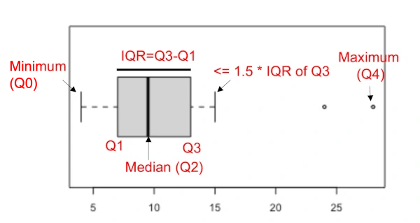
The interquartile range (IQR) is a difference between the data points which ranks at 25th percentile (first quartile or Q1) and 75th percentile (third quartile or Q3) in the dataset (IQR = Q3 - Q1).
The IQR value is used for calculating the threshold values for outlier detection,

Where, Tmin and Tmax are the thresholds for finding the outlier and c is constant which is generally 1.5 (mild outlier) or 3 (extreme outlier).
The data points which are 1.5 IQR away from Q1 and Q3 are considered as outliers. IQR method is useful when the data does not follow a normal distribution.
Create horizontal boxplot to understand IQR,
boxplot(x, horizontal = TRUE)
Calculate IQR in R,
x = c(10,4,6,8,9,8,7,6,12,14,11,9,8,4,5,10,14,12,15,7,10,14,24,28)

# get values of Q1, Q3, and IQR
summary(x)
   Min. 1st Qu.  Median    Mean 3rd Qu.    Max.
   4.00    7.00    9.50   10.62   12.50   28.00

# get IQR
IQR(x)
[1] 5.5

# get threshold values for outliers
Tmin = 7-(1.5*5.5)
Tmax = 12.50+(1.5*5.5)

# find outlier
x[which(x < Tmin | x > Tmax)]
[1] 24 28

# remove outlier
x[which(x > Tmin & x < Tmax)]
[1] 10  4  6  8  9  8  7  6 12 14 11  9  8  4  5 10 14 12 15  7 10 14
Based on IQR method, the values 24 and 28 are outliers in the dataset.
Dixon’s Q Test
The Dixon’s Q test is a hypothesis-based test used for identifying a single outlier (minimum or maximum value) in a univariate dataset.
This test is applicable to a small sample dataset (the sample size is between 3 and 30) and when data is normally distributed. Although Dixon’s Q test assumes normality, it is robust to departure from normality.
Dixon’s Q test analyzes the following hypothesis,
Null hypothesis (H0): The maximum or minimum value is not an outlier (there is no outliers)
Alternate hypothesis (Ha): The maximum or minimum value is an outlier (there is an outlier)
The null hypothesis is rejected when the Q statistics is greater than the critical Q value (theoretical Q which is expected to occur at a 5% significance level and given sample size). There are multiple variants of Dixon’s Q test based on the sample sizes.
Perform Dixon’s Q test in R,
library(outliers)
x = c(10,4,6,8,9,8,7,6,12,14,11,9,8,4,5,10,14,12,15,7,10,14,24,28)

dixon.test(x)
	Dixon test for outliers

data:  x
Q = 0.56522, p-value < 2.2e-16
alternative hypothesis: highest value 28 is an outlier
As the p value is significant (Q = 0.56, p< 2.2e-16), the maximum value 28 is an outlier.
Check if minimum value is an outlier,
dixon.test(x, opposite = TRUE)
	Dixon test for outliers

data:  x
Q = 0.090909, p-value = 0.2841
alternative hypothesis: lowest value 4 is an outlier
As the p value is not significant (Q = 0.09, p = 0.2841), the minimum value 4 is not an outlier.
Note: Dixon’s Q test works well when there is a single outlier in the dataset. This test suffers from masking (when there are multiple outliers) and swamping issues, and hence should be complemented with graphical methods such as boxplot or histogram for outlier detection.
Grubb’s Test
Grubb’s test is used for identifying a single outlier (minimum or maximum value in a dataset) in a univariate dataset. In contrast to Dixon’s Q Test, Grubb’s test should be used when sample size (n) > 6, and data is normally distributed. If n ≤ 6, Grubb’s test may find non-outliers as outliers.
Null hypothesis (H0): The maximum or minimum value is not an outlier (there is no outlier)
Alternate hypothesis (Ha): The maximum or minimum value is an outlier (there is an outlier)
The null hypothesis is rejected when the G statistics is greater than the critical G value (theoretical G which is expected to occur at a 5% significance level and given sample size).
Perform Grubb’s test in R,
library(outliers)
x = c(10,4,6,8,9,8,7,6,12,14,11,9,8,4,5,10,14,12,15,7,10,14,24,28)

grubbs.test(x)
# output
	Grubbs test for one outlier

data:  x
G = 3.0354, U = 0.5820, p-value = 0.007692
alternative hypothesis: highest value 28 is an outlier
As the p value is significant (G = 3.0354, p = 0.007692), the maximum value 28 is an outlier.
Check if minimum value is an outlier,
grubbs.test(x, opposite = TRUE)
# output
	Grubbs test for one outlier

data:  x
G = 1.15737, U = 0.93923, p-value = 1
alternative hypothesis: lowest value 4 is an outlier
As the p value (> 0.05) is not significant (G = 1.15, p = 1), the minimum value 4 is not an outlier.
If you have more than one outlier in the dataset, then you can perform multiple tests to remove outliers. You need to remove the outlier identified in each step and repeat the process.
Similar to Dixon’s Q test, Grubb’s test suffers from the masking effect.
Rosner’s test [generalized (extreme Studentized deviate) ESD many-outliers test]
Rosner’s test or generalized ESD many-outliers test (GESD) is useful to identify multiple outliers in the univariate dataset. The number of outliers in the dataset is unknown and the upper limit (k) of outliers need to be provided prior to this test.
Rosner’s test is adequately accurate for detecting up to 10 outliers when the sample size is at least 25, and data (after excluding outlier) should be normally distributed.
Rosner’s test avoid the issue masking effect (outlier is not detected due to presence of other outlier) that occurs in single outlier tests (Dixon’s Q and Grubb’s test).
Rosner’s test hypotheses,
Null hypothesis (H0): There are no outliers in the dataset
Alternate hypothesis (Ha): There are upto k potential outliers in the dataset
Perform Rosner’s test using EnvStats R package,
library(EnvStats)
# the parameter k defines the number of potential outlier in a dataset.
# the default k value is 3
rosnerTest(x, k = 2)$all.stats
# output
 i    Mean.i     SD.i Value Obs.Num    R.i+1 lambda.i+1 Outlier
1 0 10.625000 5.724186    28      24 3.035366   2.801551    TRUE
2 1  9.869565 4.465060    24      23 3.164669   2.780277    TRUE
Rosner’s test identified two outliers in the dataset (24 and 28). The value column indicates the outlier data point and
Outlier column indicates the True value if the outlier is present.
Chi-squared test for outliers
The Chi-squared test for outliers can be used for single outlier detection in the input dataset. The presence of outliers in the dataset can give large Chi-squared test statistics and hence a signifcant p value.
The Chi-squared test for outliers assumes population variance is known. If it is not provided, the variances are estimated from the sample dataset. It tests the null hypothesis that the highest (or lowest) value is not an outlier versus the alternative hypothesis that the highest (or lowest) value is an outlier.
You can perform a Chi-squared test for outliers using chisq.out.test() function in R. With default parameters, it checks
whether the highest value is an outlier or not.
library(outliers)
x = c(10,4,6,8,9,8,7,6,12,14,11,9,8,4,5,10,14,12,15,7,10,14,24,28)

chisq.out.test(x)
# output
	chi-squared test for outlier

data:  x
X-squared = 9.2134, p-value = 0.002402
alternative hypothesis: highest value 28 is an outlier
As the p value from the Chi-squared test for an outlier is significant (χ2 = 9.21, p = 0.002), we reject the null hypothesis and conclude that the highest value 28 is an outlier.
If you want to test whether the lowest value is an outlier, you can set the opposite = TRUE,
chisq.out.test(x, opposite = TRUE)

	chi-squared test for outlier

data:  x
X-squared = 1.3395, p-value = 0.2471
alternative hypothesis: lowest value 4 is an outlier
As the p value from the Chi-squared test for an outlier is not significant (χ2 = 1.33, p = 0.24), we fail to reject the null hypothesis and conclude that the lowest value 4 is not an outlier.
Chi-squared test for outliers is not a recommended test for outlier detection as other well performing tests exists for outlier analysis (see above in this article).
Note: The identification of outliers in a dataset is a tricky process. Before finding outliers, it is good to know the source of outliers and why they are present in the dataset. If the outlier data point is a part of underlying treatment response such as biological variation of the samples, it should be investigated.
When it comes to outlier identification and removal, it is better to use multiple methods to identify outliers. For example, the statistical methods should be complemented with visual approaches for outlier identification.
Enhance your skills with courses on Statistics and R
- Introduction to Statistics
- R Programming
- Data Science: Foundations using R Specialization
- Data Analysis with R Specialization
- Getting Started with Rstudio
- Applied Data Science with R Specialization
- Statistical Analysis with R for Public Health Specialization
References
- Yang J, Rahardja S, Fränti P. Outlier detection: how to threshold outlier scores?. InProceedings of the international conference on artificial intelligence, information processing and cloud computing 2019 Dec 19 (pp. 1-6).
- Evaluating Analytical Data
- Rosner B. Percentage points for a generalized ESD many-outlier procedure. Technometrics. 1983 May 1;25(2):165-72.
- Generalized ESD Test for Outliers
If you have any questions, comments, corrections, or recommendations, please email me at reneshbe@gmail.com
This work is licensed under a Creative Commons Attribution 4.0 International License
Some of the links on this page may be affiliate links, which means we may get an affiliate commission on a valid purchase. The retailer will pay the commission at no additional cost to you.

