Friedman test using R (with examples and code)

What is Friedman test?

• Friedman test (Friedman Rank Sum test) is a nonparametric alternative to one-way repeated measure ANOVA. Friedman test is not a nonparametric equivalent to two-way ANOVA.
• Friedman test is appropriate when a sample does not meet the assumption of normality or dependent variable is measured on an ordinal scale (e.g. Likert scale).
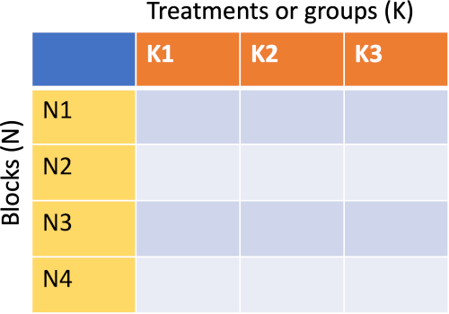
• Friedman test compares the differences between three or more paired treatments (groups) where two-way (treatments and blocks/individuals) data is arranged in randomized complete block design or repeated measure design. The data inside the block is unreplicated (only one observation for each treatment).
• In Friedman test, the ranks for each subject (within a block) are arranged from lowest to highest, and the sum of ranks are compared for each treatment.

Assumptions of Friedman test

• Dependent variable should be measured on a continuous or ordinal scale
• Treatments are random sample from population
• The observations in blocks should be mutually independent (results from one block should not affect the results from other block)
• There should be three or more treatments
• There is no interactions between the treatment and blocks
• Data do not need to meet the assumption of parametric test (e.g. normality)

Friedman test formula

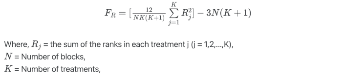
Under the null hypothesis, the Friedman’s test follows the χ2 distribution with K-1 degree of freedoms when the sample size is large (N > 15 or K > 5)

Friedman test Hypotheses

• Null hypothesis: The treatment have equal effect
• Alternative hypothesis: At least one treatment effect is different from other treatment effect

Learn more about hypothesis testing and interpretation

Friedman test example and analysis in R

A researcher wants to evaluate the efficacy of different plant varieties on bacterial disease severity at different locations. The dependent variable is the disease severity index measured on an ordinal scale (1 to 5, with 1 being no disease and 5 being severe disease symptoms). Plant varieties and locations are independent variables. To check whether locations have an effect on disease severity on each plant variety, the researcher evaluated the disease severity index for each plant variety at different locations.

Load the dataset

library(tidyverse)
df=read_csv("https://reneshbedre.github.io/assets/posts/anova/plant_disease_friedman.csv")
head(df, 2)
# output
 Id       L1    L2    L3    L4
  <chr> <dbl> <dbl> <dbl> <dbl>
1 P1        4     2     5     4
2 P2        3     1     4     3

# make it in long format
df_long <- df %>% gather(key = "locations", value = "disease", L1, L2, L3, L4)
# output
  plant_var locations disease
  <chr>     <chr>       <dbl>
1 P1        L1              4
2 P2        L1              3

Summary statistics and visualization of dataset

Get summary statistics based on dependent variable and covariate,

df_long %>% group_by(locations) %>%  summarise(n = n(), mean = mean(disease), 
                                               sd = sd(disease))
# output
 locations     n  mean    sd
  <chr>     <int> <dbl> <dbl>
1 L1            5   4.2 0.837
2 L2            5   1.4 0.548
3 L3            5   4   0.707
4 L4            5   4   0.707

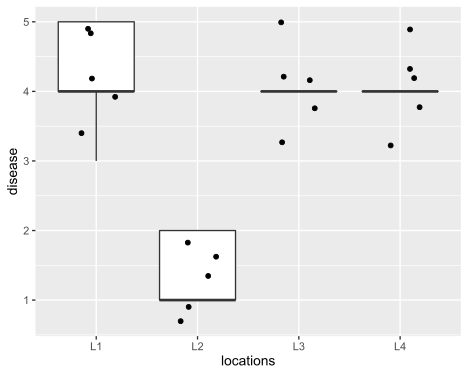
Visualize dataset,

ggplot(df_long, aes(x = locations, y = disease)) + geom_boxplot(outlier.shape = NA) + 
    geom_jitter(width = 0.2) + theme(legend.position="top")

perform Friedman test

We will use the friedman.test function from stats package to perform Friedman test

Pass the following parameters to friedman.test function,

• y : numeric vector of dependent variable or a data matrix
• groups : a vector of treatment (K) variable (ignored if y is a matrix)
• blocks : a vector of block (N) variable (ignored if y is a matrix)
• formula : Specify the formula of the form a ~ b | c, where a (dependent variable), b (treatment) and c (blocks)
• data : data frame or matrix for formula

library(stats)
friedman.test(y = df_long$disease, groups = df_long$locations, blocks = df_long$plant_var)
# same as friedman.test(formula = disease ~ locations | plant_var, data = df_long)
# output
	Friedman rank sum test

data:  df_long$disease, df_long$locations and df_long$plant_var
Friedman chi-squared = 9.8478, df = 3, p-value = 0.0199

Friedman test results indicate that there are significant differences [χ2(3) = 9.84, p = 0.01] in disease severity in plant varieties based on their locations.

Check how to perform Friedman test in Python

Friedman test effect size

Kendall’s coefficient of concordance (Kendall’s W) can be used for measuring the effect size (degree of difference) for the Friedman test.

library(rstatix)
df_long %>% friedman_effsize(disease ~ locations | plant_var)
# output
  .y.         n effsize method    magnitude
* <chr>   <int>   <dbl> <chr>     <ord>    
1 disease     5   0.657 Kendall W large

Kendall’s W is 0.657 and indicates a large effect size. Kendall’s W is based on Cohen’s interpretation guidelines (0.1: small effect; 0.3: moderate effect; and >0.5: large effect).

post-hoc test

Friedman test is an omnibus test statistic, which indicates that there are significant differences in disease severity in plant varieties based on locations but does not tell which locations have a significant effect on disease severity.

To know which locations are significantly different, you need to use Conover’s test tests for pairwise comparisons of locations. In addition to Conover’s test, Wilcoxon-Nemenyi-McDonald-Thompson test (Nemenyi test) can also be used as post-hoc test for significant Friedman test.

The Bonferroni correction will be used to adjust the p values for multiple hypothesis testing at a 5% cut-off

Let’s perform the Conover’s test using frdAllPairsConoverTest function from PMCMRplus package,

Pass the following parameters to frdAllPairsConoverTest function,

• y : numeric vector of dependent variable
• groups : a vector of treatment (K) variable
• blocks : a vector of block (N) variable
• p.adjust.method : method for p value adjustment

library(PMCMRplus)

frdAllPairsConoverTest(y = df_long$disease, groups = df_long$locations, 
                        blocks = df_long$plant_var, p.adjust.method = "bonf")
# output
Pairwise comparisons using Conover all-pairs test for a two-way balanced complete block design

data: y, groups and blocks

   L1   L2   L3  
L2 0.13 -    -   
L3 1.00 0.17 -   
L4 1.00 0.21 1.00

P value adjustment method: bonferroni

The multiple pairwise comparisons from Conover’s test suggest that there are no statistically significant differences between different locations on disease severity for different plant varieties, despite there being low disease severity for location L2.

Enhance your skills with courses on statistical analysis and R

• Designing, Running, and Analyzing Experiments
• Statistics with R Specialization
• Data Science: Foundations using R Specialization
• Getting Started with Rstudio

Related reading

• MANOVA using R (with examples and code)
• What is p value and how to calculate p value by hand
• Repeated Measures ANOVA using Python and R (with examples)
• ANOVA using Python (with examples)
• Multiple hypothesis testing problem in Bioinformatics

References

• Bewick V, Cheek L, Ball J. Statistics review 10: further nonparametric methods. Critical care. 2004 Jun;8(3):1- 4..
• Kim HY. Statistical notes for clinical researchers: Nonparametric statistical methods: 2. Nonparametric methods for comparing three or more groups and repeated measures. Restorative Dentistry and Endodontics. 2014;39(4):329- 32.
• Friedman test in SPSS.
• Friedman test
• Salvatore S. Mangiafico. Friedman Test

If you have any questions, comments or recommendations, please email me at reneshbe@gmail.com

This work is licensed under a Creative Commons Attribution 4.0 International License

Some of the links on this page may be affiliate links, which means we may get an affiliate commission on a valid purchase. The retailer will pay the commission at no additional cost to you.