Kruskal-Wallis test in R [with example and code]
Kruskal-Wallis (KW) test
- Kruskal-Wallis test (also known as Kruskal-Wallis H test or Kruskal–Wallis ANOVA) is a non-parametric (distribution free) alternative to the one-way ANOVA.
- Kruskal-Wallis test is useful when the assumptions of ANOVA are not met or there is a significant deviation from the ANOVA assumptions. If the data meets the ANOVA assumptions, it is better to use ANOVA as it is a little more powerful than non-parametric tests.
- Kruskal-Wallis test used for comparing the differences between two or more groups. It is an extension to the Mann Whitney U Test, which is used for comparing two groups. It compares the mean ranks (medians) of groups.
- Kruskal-Wallis test does not assume any specific distribution (such as normal distribution of samples) for calculating test statistics and p values.
- The sample mean ranks or medians are compared in the Kruskal-Wallis test, which distinguishes it from the ANOVA, which compares sample means. Medians are less sensitive to outliers than means.
Kruskal-Wallis test assumptions
- The independent variable should have two or more independent groups
- The observations from the independent groups should be randomly selected from the target populations
- Observations are sampled independently from each other (no relation in observations between the groups and within the groups) i.e., each subject should have only one response
- The dependent variable should be continuous or ordinal (e.g. Likert item data)
Kruskal-Wallis test Hypotheses
If each group distribution is not same,
Null hypothesis: All group mean ranks are equal
Alternative hypothesis: At least, one group mean rank different from other groups
In terms of medians (when each group distribution is same),
Null hypothesis: Populations medians are equal
Alternative hypothesis: At least, one population median is different from other populations
Learn more about hypothesis testing and interpretation
Kruskal-Wallis test formula
Kruskal-Wallis test statistics (H) is given as,
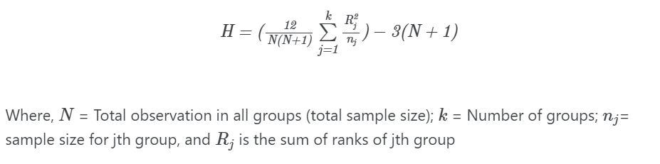
H is approximately chi-squared distributed with k-1 degress of freedom
The p value is calculated based on the comparison between the critical value and the H value. If H >= critical value, we reject the null hypothesis and vice versa.
As the Kruskal-Wallis test is based on the chi-squared distribution, the sample size for each group should be at least five.
Perform Kruskall-Wallis test in R
Get example dataset
Assume we have three plant varieties, each with a different yield value. We need to see whether there are any significant differences in yield across the three plant varieties in this dataset.
Kruskal-Wallis test can be performed on a dataset with unequal sample size in each group
Load and visualize dataset,
Learn how to import data using pandas
library(tidyverse)
df = read.csv("https://reneshbedre.github.io/assets/posts/mann_whitney/genotype_kw.csv")
head(df, 2)
   plant_var yield
1          A    70
2          A    20
Summary statistics,
df %>% group_by(plant_var) %>%  summarise(n = n(), mean = mean(yield), sd = sd(yield))
# output
  plant_var     n  mean    sd
  <chr>     <int> <dbl> <dbl>
1 A             5    35  27.8
2 B             5    90   0
3 C             5    20   0
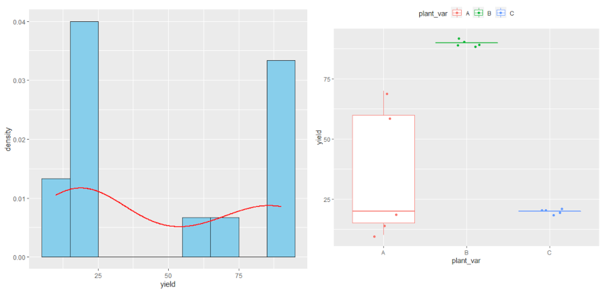
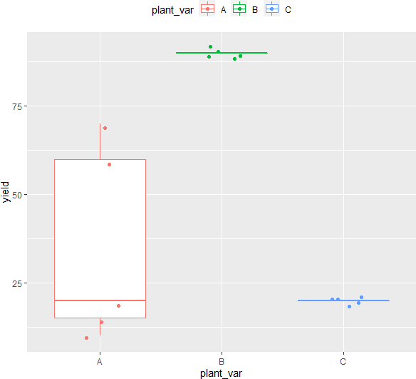
Generate boxplot to check data spread
ggplot(df, aes(x = plant_var, y = yield, col = plant_var)) + geom_boxplot(outlier.shape = NA) + geom_jitter(width = 0.2) + theme(legend.position="top")
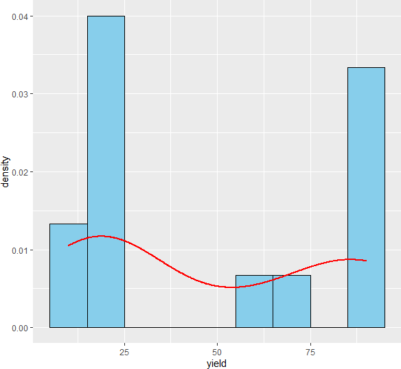
Check data distribution
Check data distribution and normality assumptions using Shapiro-Wilk test and histogram ,
shapiro.test(df$yield)
# output
	Shapiro-Wilk normality test

data:  df$yield
W = 0.75495, p-value = 0.001027

# plot histogram
ggplot(df, aes(x = yield)) + geom_histogram(aes(y=..density..), colour="black", fill="skyblue", binwidth = 10) +
    geom_density(color="red", size=1)
Check homogeneity of variances assumption,
library(car)
leveneTest(yield ~ plant_var, data=df)
Levene's Test for Homogeneity of Variance (center = median)
      Df F value Pr(>F)
group  2  4.3663 0.0376 *
      12
As the p value obtained from the Shapiro-Wilk test and Levene’s test is significant (p < 0.05), we conclude that the data is not normally distributed and does not have equal variance. Further, in histogram data distribution shape does not look normal. Therefore, the parametric test ANOVA may not be appropriate here. Kruskal-Wallis test is more appropriate for analyzing differences among three plant varieties.
Perform Kruskal-Wallis test
kruskal.test(yield ~ plant_var, data = df)
# output
	Kruskal-Wallis rank sum test

data:  yield by plant_var
Kruskal-Wallis chi-squared = 10.396, df = 2, p-value = 0.005527

# calculate effect size
library(rcompanion)
epsilonSquared(x = df$yield, g = df$plant_var)
# output
epsilon.squared
          0.743
As the p value obtained from the Kruskal-Wallis test test is significant (H (2) = 10.39, p < 0.05), we conclude that there are significant differences in yield among the plant varieties.
For the Kruskal-Wallis test, epsilon-squared is a method of choice for effect size measurement. The epsilon-squared is 0.74 and suggests a very strong effect of plant varieties on yield.
epsilon-squared > 0.64 suggest very strong effect. Read more about epsilon-squared scale
post-hoc test
Kruskal-Wallis test is an omnibus test statistics, which indicates that there are significant differences in yield among the plant varieties, but does not tell which plant varieties are different from each other.
To know which plant varieties are significantly different from each other, we will perform the Dunn’s test as post-hoc test for significant Kruskal-Wallis test. As there are multiple comparisons, we will correct the p values using Benjamini-Hochberg FDR method for multiple hypothesis testing at a 5% cut-off.
The other tests that can be used for post-hoc test includes Conover and Nemenyi tests.
Dunn’s test is more appropriate post-hoc than the Mann-Whitney U test for significant Kruskal-Wallis test as it retains the rank sums of the Kruskal-Wallis.
library(FSA)
dunnTest(yield ~ plant_var, data = df, method = "bh")
# output
Dunn (1964) Kruskal-Wallis multiple comparison
  p-values adjusted with the Benjamini-Hochberg method.

  Comparison         Z     P.unadj       P.adj
1      A - B -2.792316 0.005233219 0.007849829
2      A - C  0.000000 1.000000000 1.000000000
3      B - C  2.792316 0.005233219 0.015699657
Let’s check the results with additional Conover and Nemenyi tests post-hoc tests,
Conover test,
library(PMCMRplus)
df$plant_var = as.factor(df$plant_var)
# Tukey's p-adjustment (single-step method)
kwAllPairsConoverTest(yield ~ plant_var, data = df)

# output
	Pairwise comparisons using Conover all-pairs test

data: yield by plant_var

  A       B
B 0.00071 -
C 1.00000 0.00071

P value adjustment method: single-step
Nemenyi test,
# Nemenyi test
# Tukey's p-adjustment (single-step method)
kwAllPairsNemenyiTest(yield ~ plant_var, data = df)
# output
	Pairwise comparisons using Tukey-Kramer-Nemenyi all-pairs test with Tukey-Dist approximation

data: yield by plant_var

  A     B
B 0.022 -
C 1.000 0.022

P value adjustment method: single-step
The post-hoc test using the Dunn test indicates that there are significant differences in yield between A and B (p adjusted < 0.01) and B and C (p adjusted < 0.05) plant varieties. It appears that the B plant variety has a significantly higher yield than the A and C plant varieties.
Enhance your skills with statistical courses using R
References
- Hecke TV. Power study of anova versus Kruskal-Wallis test. Journal of Statistics and Management Systems. 2012 May 1;15(2-3):241-7.
- Tests with More than Two Independent Samples
- Hazra A, Gogtay N. Biostatistics series module 3: comparing groups: numerical variables. Indian journal of dermatology. 2016 May;61(3):251.
- Dinno A. Nonparametric pairwise multiple comparisons in independent groups using Dunn’s test. The Stata Journal. 2015 Apr;15(1):292-300.
If you have any questions, comments or recommendations, please email me at reneshbe@gmail.com
This work is licensed under a Creative Commons Attribution 4.0 International License
Some of the links on this page may be affiliate links, which means we may get an affiliate commission on a valid purchase. The retailer will pay the commission at no additional cost to you.

