How to Perform MANOVA in R
What is MANOVA?
MANOVA (Multivariate Analysis of Variance) is a statistical method that analyzes the differences among multiple groups across multiple dependent variables.
MANOVA is an extension to univariate ANOVA. The main difference between ANOVA and MANOVA is that ANOVA compares group means based on one dependent variables (univariate ANOVA), whereas MANOVA compares group means based on two or more dependent variables (Multivariate ANOVA).
MANOVA is useful when there are multiple dependent variables and they are inter-correlated. While analyzing the differences among groups, MANOVA reduces the type I error which can be inflated by performing separate univariate ANOVA for each dependent variable.
Assumptions of MANOVA
MANOVA follows similar assumptions as in ANOVA for the independence of observations and homogeneity of variances.
In addition, MANOVA needs to meet the following assumption,
- Multivariate normality: data or residuals should have a multivariate normal distribution for each combination of independent and dependent variables (checked by Shapiro-Wilk test for univariate normality and Mardia’s skewness and kurtosis for multivariate normality)
- Homogeneity of the variance-covariance matrices: data should have equal variance-covariance matrices for each combination formed by each group in the independent variable. This is a multivariate version of the Homogeneity of variances that is checked in univariate ANOVA. It can be tested using Box’s M test. Box’s M-test has little power and uses a lower alpha level such as 0.001 to assess the p value for significance.
- Multicollinearity: There should be no multicollinearity (very high correlations i.e., > 0.9) among dependent variables
- Linearity: dependent variables should be linearly related for each group of the independent variable. If there are more than two dependent variables, the pair of dependent variables should be linearly related
- There should be no outliers in the dependent variables (multivariate outliers) (checked by Mahalanobis distances)
- dependent variables should be continuous
MANOVA Hypotheses
- Null hypothesis (H0): group mean vectors are same for all groups
- Alternative hypothesis (H1): group mean vectors are not same for all groups
One-way (one factor) MANOVA in R
In one-way MANOVA, there is one independent variable with two or more groups and at least two dependent variables.
One-way MANOVA is an extension to one-way ANOVA and handles the multiple correlated dependent variables simultaneously.
MANOVA example dataset
Suppose we have a dataset of various plant varieties (plant_var) and their associated phenotypic measurements for
plant heights (height) and canopy volume (canopy_vol). We want to see if plant heights and canopy volume are
associated with different plant varieties using MANOVA.
For MANOVA, the dataset should contain more observations per group in independent variables than a number of the dependent variables. It is particularly important for testing the Homogeneity of the variance-covariance matrices using Box’s M-test.
Load dataset,
# load package
library(tidyverse)

# load dataset
df=read_csv("https://reneshbedre.github.io/assets/posts/ancova/manova_data.csv")

# view first 2 rows
head(df, 2)
# output
  plant_var height canopy_vol
  <chr>      <dbl>      <dbl>
1 A             20        0.7
2 A             22        0.8
Summary statistics and visualization of dataset
Get summary statistics based on each dependent variable,
# summary statistics for dependent variable height
df %>% group_by(plant_var) %>%  summarise(n = n(), mean = mean(height), sd = sd(height))
# output
 plant_var     n  mean    sd
  <chr>     <int> <dbl> <dbl>
1 A            10 18.9   2.92
2 B            10 16.5   1.92
3 C            10  3.05  1.04
4 D            10  9.35  2.11

# summary statistics for dependent variable canopy_vol
df %>% group_by(plant_var) %>%  summarise(n = n(), mean = mean(canopy_vol), sd = sd(canopy_vol))
# output
  plant_var     n  mean     sd
  <chr>     <int> <dbl>  <dbl>
1 A            10 0.784 0.121
2 B            10 0.608 0.0968
3 C            10 0.272 0.143
4 D            10 0.474 0.0945
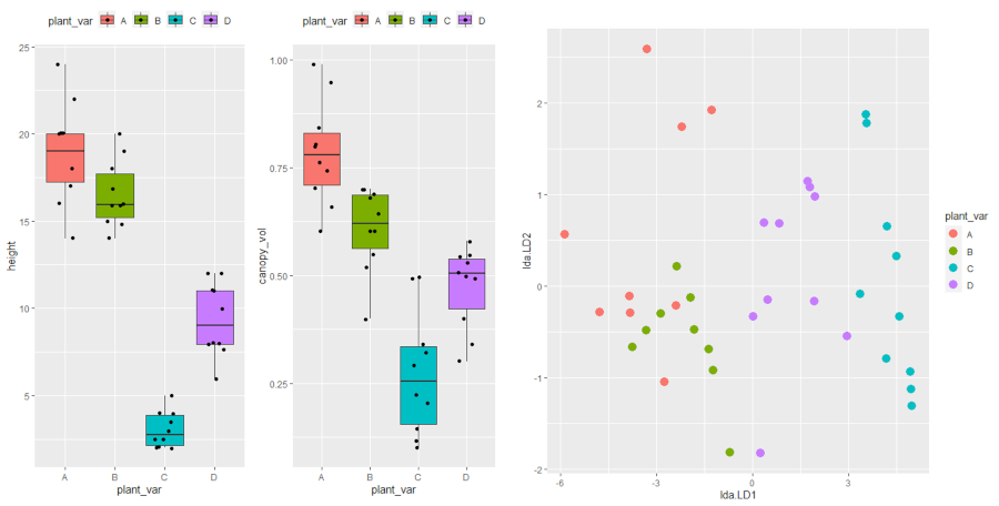
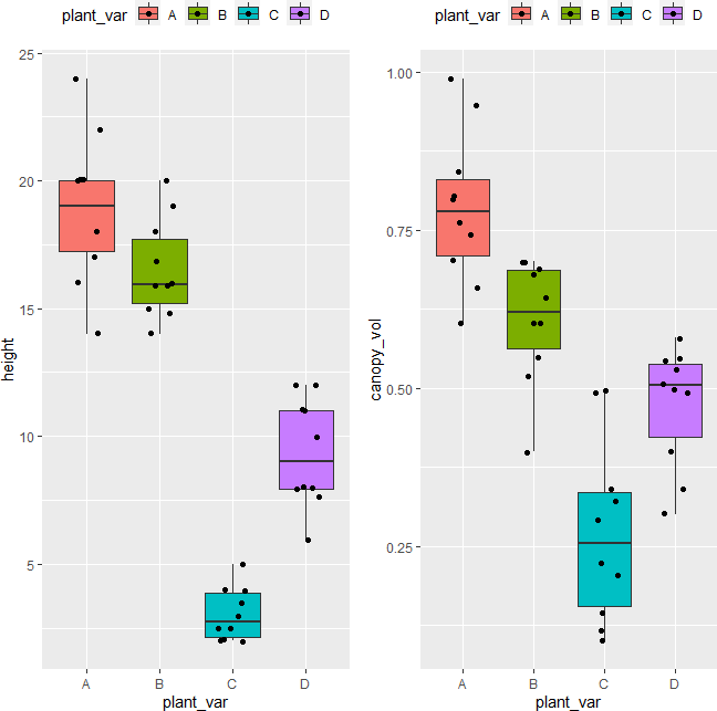
Visualize dataset,
# load package
library(gridExtra)

p1 <- ggplot(df, aes(x = plant_var, y = height, fill = plant_var)) + geom_boxplot(outlier.shape = NA) + geom_jitter(width = 0.2) + theme(legend.position="top")
p2 <- ggplot(df, aes(x = plant_var, y = canopy_vol, fill = plant_var)) + geom_boxplot(outlier.shape = NA) + geom_jitter(width = 0.2) + theme(legend.position="top")
grid.arrange(p1, p2, ncol=2)
perform one-way MANOVA
dep_vars <- cbind(df$height, df$canopy_vol)

# fir the model
fit <- manova(dep_vars ~ plant_var, data = df)
summary(fit)
# output
          Df Pillai approx F num Df den Df    Pr(>F)
plant_var  3 1.0365   12.909      6     72 7.575e-10 ***
Residuals 36

# get effect size
library(effectsize)
effectsize::eta_squared(fit)
# output
Parameter | Eta2 (partial) |       95% CI
-----------------------------------------
plant_var |           0.52 | [0.36, 1.00]
The Pillai’s Trace test statistics is statistically significant [Pillai’s Trace = 1.03, F(6, 72) = 12.90, p < 0.001] and indicates that plant varieties has a statistically significant association with both combined plant height and canopy volume.
The measure of effect size (Partial Eta Squared; ηp2) is 0.52 and suggests that there is a large effect of plant varieties on both plant height and canopy volume.
post-hoc test
The MANOVA results suggest that there are statistically significant (p < 0.001) differences between plant varieties, but it does not tell which groups are different from each other. To know which groups are significantly different, the post-hoc test needs to carry out.
To test the between-group differences, the univariate ANOVA can be done on each dependent variable, but this will be not appropriate and lose information that can be obtained from multiple variables together.
Here we will perform the linear discriminant analysis (LDA) to see the differences between each group. LDA will discriminate the groups using information from both the dependent variables.
library(MASS)
post_hoc <- lda(df$plant_var ~ dep_vars, CV=F)
post_hoc
# output
Call:
lda(df$plant_var ~ dep_vars, CV = F)

Prior probabilities of groups:
   A    B    C    D
0.25 0.25 0.25 0.25

Group means:
  dep_vars1 dep_vars2
A     18.90     0.784
B     16.54     0.608
C      3.05     0.272
D      9.35     0.474

Coefficients of linear discriminants:
                 LD1        LD2
dep_vars1 -0.4388374 -0.2751091
dep_vars2 -1.3949158  9.3256280

Proportion of trace:
   LD1    LD2
0.9855 0.0145

# plot
plot_lda <- data.frame(df[, "plant_var"], lda = predict(post_hoc)$x)
ggplot(plot_lda) + geom_point(aes(x = lda.LD1, y = lda.LD2, colour = plant_var), size = 4)
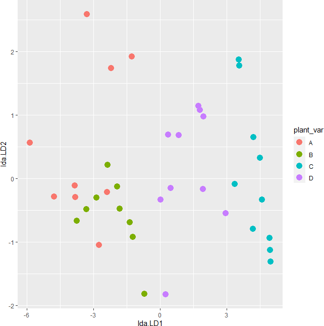
The LDA scatter plot discriminates against multiple plant varieties based on the two dependent variables. The C and D plant variety has a significant difference (well separated) as compared to A and B. A and B plant varieties are more similar to each other. Overall, LDA discriminated between multiple plant varieties.
Test MANOVA assumptions
Assumptions of multivariate normality
This test may not be easy to test as it may not be available in all statistical software packages. You can initially check the univariate normality for each combination of the independent and dependent variables. If this test does not pass (significant p value), it may be possible that multivariate normality is violated.
Note: As per Multivariate Central Limit Theorem, if the sample size is large (say n > 20) for each combination of the independent and dependent variable, we can assume the assumptions of multivariate normality.
library(rstatix)
df %>% group_by(plant_var) %>%  shapiro_test(height, canopy_vol)
 plant_var variable   statistic     p
  <chr>     <chr>          <dbl> <dbl>
1 A         canopy_vol     0.968 0.876
2 A         height         0.980 0.964
3 B         canopy_vol     0.882 0.137
4 B         height         0.939 0.540
5 C         canopy_vol     0.917 0.333
6 C         height         0.895 0.194
7 D         canopy_vol     0.873 0.109
8 D         height         0.902 0.231
As the p value is non-significant (p > 0.05) for each combination of independent and dependent variable, we fail to reject the null hypothesis and conclude that data follows univariate normality.
If the sample size is large (say n > 50), the visual approaches such as QQ-plot and histogram will be better for assessing the normality assumption. Read more here
Now, let’s check for multivariate normality using Mardia’s Skewness and Kurtosis test,
library(mvnormalTest)
mardia(df[, c("height", "canopy_vol")])$mv.test
# output
          Test Statistic p-value Result
1     Skewness    2.8598  0.5815    YES
2     Kurtosis   -0.9326   0.351    YES
3 MV Normality      <NA>    <NA>    YES
As the p value is non-significant (p > 0.05) for Mardia’s Skewness and Kurtosis test, we fail to reject the null hypothesis and conclude that data follows multivariate normality.
Here both Skewness and Kurtosis p value should be > 0.05 for concluding the multivariate normality.
Homogeneity of the variance-covariance matrices
We will use Box’s M test to assess the homogeneity of the variance-covariance matrices. Null hypothesis: variance-covariance matrices are equal for each combination formed by each group in the independent variable
library(heplots)
boxM(Y = df[, c("height", "canopy_vol")], group = df$plant_var)
# output
	Box M-test for Homogeneity of Covariance Matrices

data:  df[, c("height", "canopy_vol")]
Chi-Sq (approx.) = 21.048, df = 9, p-value = 0.01244
As the p value is non-significant (p > 0.001) for Box’s M test, we fail to reject the null hypothesis and conclude that variance-covariance matrices are equal for each combination of dependent variable formed by each group in independent variable.
If this assumption fails, it would be good to check the homogeneity of variance assumption using Bartlett’s or Levene’s test to identify which variable fails in equal variance.
Multivariate outliers
MANOVA is highly sensitive to outliers and may produce type I or II errors. Multivariate outliers can be detected using the Mahalanobis Distance test. The larger the Mahalanobis Distance, the more likely it is an outlier.
library(rstatix)
# get distance
mahalanobis_distance(data = df[, c("height", "canopy_vol")])$is.outlier
# output
 [1] FALSE FALSE FALSE FALSE FALSE FALSE FALSE FALSE FALSE FALSE FALSE FALSE FALSE FALSE FALSE FALSE FALSE
[18] FALSE FALSE FALSE FALSE FALSE FALSE FALSE FALSE FALSE FALSE FALSE FALSE FALSE FALSE FALSE FALSE FALSE
[35] FALSE FALSE FALSE FALSE FALSE FALSE
From the results, there is no multivariate outliers (all is.outlier = FALSE or p > 0.001) in the dataset. If is.outlier = TRUE, it means there is multivariate outlier in the dataset.
Linearity assumption
Linearity assumption can be checked by visualizing the pairwise scatterplot for the dependent variable for each group. The data points should lie on the straight line to meet the linearity assumption. The violation of the linearity assumption reduces the statistical power.
library(gridExtra)
p1 <- df  %>% group_by(plant_var) %>% filter(plant_var == "A") %>% ggplot(aes(x = height, y = canopy_vol)) + geom_point() + ggtitle("Variety: A")
p2 <- df  %>% group_by(plant_var) %>% filter(plant_var == "B") %>% ggplot(aes(x = height, y = canopy_vol)) + geom_point() + ggtitle("Variety: B")
p3 <- df  %>% group_by(plant_var) %>% filter(plant_var == "C") %>% ggplot(aes(x = height, y = canopy_vol)) + geom_point() + ggtitle("Variety: C")
p4 <- df  %>% group_by(plant_var) %>% filter(plant_var == "D") %>% ggplot(aes(x = height, y = canopy_vol)) + geom_point() + ggtitle("Variety: D")
grid.arrange(p1, p2, p3, p4, ncol=2)
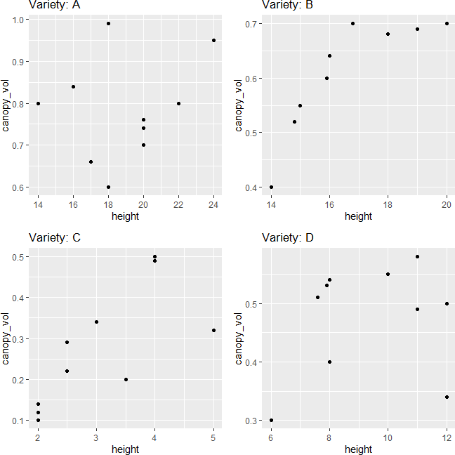
The scatterplot indicates that dependent variables have a linear relationship for each group in the independent variable
Multicollinearity assumption
Multicollinearity can be checked by correlation between the dependent variable. If you have more than two dependent variable you can use correlation matrix or variance inflation factor to assess the multicollinearity.
The correlation between the dependent variable should not be> 0.9 or too low. If the correlation is too low, you can perform separate univariate ANOVA for each dependent variable.
cor.test(x = df$height, y = df$canopy_vol, method = "pearson")$estimate
# output
      cor
0.8652548
As the correlation coefficient between the dependent variable is < 0.9, there is no multicollinearity.
Related article: MANOVA in Python
References
- Warne RT. A primer on multivariate analysis of variance (MANOVA) for behavioral scientists. Practical Assessment, Research & Evaluation. 2014 Nov 1;19.
- Mardia KV. Measures of multivariate skewness and kurtosis with applications. Biometrika. 1970 Dec 1;57(3):519-30.
- French A, Macedo M, Poulsen J, Waterson T, Yu A. Multivariate analysis of variance (MANOVA).
- Multivariate Central Limit Theorem
Enhance your skills with courses on Statistics and R
- Introduction to Statistics
- R Programming
- Data Science: Foundations using R Specialization
- Data Analysis with R Specialization
- Getting Started with Rstudio
- Applied Data Science with R Specialization
- Statistical Analysis with R for Public Health Specialization
This work is licensed under a Creative Commons Attribution 4.0 International License
Some of the links on this page may be affiliate links, which means we may get an affiliate commission on a valid purchase. The retailer will pay the commission at no additional cost to you.

