Linear regression in Python (using sklearn and statsmodels)

What is Linear Regression?
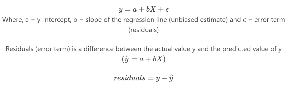
Linear regression is a supervised machine learning algorithm that models the linear relationship between
independent (X) variables and dependent variable (y). In
simple linear regression (univariate), there is one independent variable, whereas in
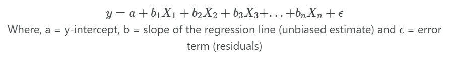
multiple linear regression, there are multiple independent variables in a model.
In regression, the independent and dependent variables are also known as features and target variables, respectively.
Once the linear regression model is fitted, the regression model is useful to predict the value of (y) based on
the given X values. A regression problem differs from a classification problem in that regression has an infinite
number of possible outcomes, while classification only has a limited number of class label outcomes.
In simple linear regression, linear relationships between y and X variables can be explained by a single X
variable
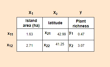
In multiple linear regression, linear relationships between Y and X variables can be explained by multiple independent (X)
variables
Note: In regression, dependent variable also called a response, outcome, regressand, criterion, or endogenous variable. Independent variable also called explanatory, covariates, predictor, regressor, exogenous, manipulated, or feature variable.
Linear Regression Assumptions
- Linear relationship: The relationship between the independent (
X) and dependent (y) variables should be linear It can be tested using the residual scatterplot (residuals vs fitted values). - Independence of residuals (errors): The residuals should be independent of each other. In case of time series data, there should be no autocorrelation (correlation between successive residuals). Autocorrelation can be tested using the Durbin-Watson test.
- Homogeneity of variance (Homoscedasticity): The residuals should have equal variance. It can be tested using the residual scatterplot (residuals vs fitted values).
- Normality: Residuals should be normally distributed. It can be tested using the Quantile-quantile (QQ) plot.
Perform simple linear regression in Python
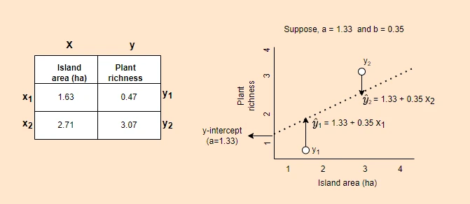
- For performing the simple linear regression, we will use the plant species richness data to study the influence of island area on the native plant richness of islands. The data is collected from 22 different coastal islands (McMaster 2005).
- The dataset contains native plant richness (
ntv_rich) as a dependent variable (y) and island area as the independent variable (X).
Load packages and dataset
To perform Linear Regression in Python, we will use statsmodels and
bioinfokit packages. If you have not installed these packages,
you can install them using pip or conda.
Now, let’s start with loading the required Python packages and the example dataset. (If you have your dataset, you
should import it as a pandas DataFrame.
from bioinfokit.analys import stat, get_data
import numpy as np
import pandas as pd

df = get_data('plant_richness_lr').data
df.head(2)
   ntv_rich      area
0  1.897627  1.602060
1  1.633468  0.477121

X = df['area']   # independent variable
y = df['ntv_rich']   # dependent variable
Fit the model
Here, we will use sklearn and statsmodels packages for linear regression analysis. sklearn focuses on prediction
analysis, while statsmodels provides detailed statistical output for linear regression analysis.
Now, fit the regression using sklearn LinearRegression()
function. It employs the ordinary least squares (OLS) method for regression analysis.
from sklearn.linear_model import LinearRegression

X = np.array(X).reshape(-1, 1) # sklearn requires in 2D array
y = np.array(y)
reg = LinearRegression().fit(X, y)

# get regression coefficient (slope)
reg.coef_
# output
array([0.35573936])

# get y intercept
reg.intercept_
# output
1.33604

# predict y (y hat) when X 2.5
reg.predict([[2.5]])
# output
array([2.22539668])
Now, fit the regression using statsmodels OLS
function, which takes the following required arguments for performing the regression analysis. In addition, you need to
explicitly add the intercept as it is not included in the model.
endog: dependent variable (y)
exog: independent variable (X)
import statsmodels.api as sm

# add intercept (optional)
X = sm.add_constant(X)

# fit the simple linear regression model
reg = sm.OLS(y, X).fit()
reg.summary()
# output

                            OLS Regression Results
==============================================================================
Dep. Variable:               ntv_rich   R-squared:                       0.828
Model:                            OLS   Adj. R-squared:                  0.819
Method:                 Least Squares   F-statistic:                     96.13
Date:                Sat, 13 Feb 2021   Prob (F-statistic):           4.40e-09
Time:                        19:56:31   Log-Likelihood:                 4.0471
No. Observations:                  22   AIC:                            -4.094
Df Residuals:                      20   BIC:                            -1.912
Df Model:                           1
Covariance Type:            nonrobust
==============================================================================
                 coef    std err          t      P>|t|      [0.025      0.975]
------------------------------------------------------------------------------
const          1.3360      0.096     13.869      0.000       1.135       1.537
area           0.3557      0.036      9.805      0.000       0.280       0.431
==============================================================================
Omnibus:                        0.057   Durbin-Watson:                   1.542
Prob(Omnibus):                  0.972   Jarque-Bera (JB):                0.278
Skew:                          -0.033   Prob(JB):                        0.870
Kurtosis:                       2.453   Cond. No.                         6.33
==============================================================================

# predict y (y hat) when X 2.5
reg.predict([[1,2.5]])
# output
array([2.22539668])
Regression metrics
The performance of the fitted regression model can be evaluated by various metrics such as Mean Squared Error (MSE), Root Mean Squared Error (RMSE), Mean absolute error (MAE), and Mean Absolute Percentage Error (MAPE). The error should be as close to zero as possible. Models with lower error metrics perform better.
Calculate the regression metrics using sklearn.metrics module functions,
from sklearn.metrics import mean_squared_error, mean_absolute_error, mean_absolute_percentage_error

# Mean Squared Error (MSE)
mean_squared_error(y_true=np.array(y), y_pred=reg.predict(X))
# output
0.0405266

# Root Mean Squared Error (RMSE)
mean_squared_error(y_true=np.array(y), y_pred=reg.predict(X), squared=False)
# output
0.201312

# Mean absolute error (MAE)
mean_absolute_error(y_true=np.array(y), y_pred=reg.predict(X))
# output
0.155394

# Mean Absolute Percentage Error (MAPE)
mean_absolute_percentage_error(y_true=np.array(y), y_pred=reg.predict(X))
# output
0.0853556
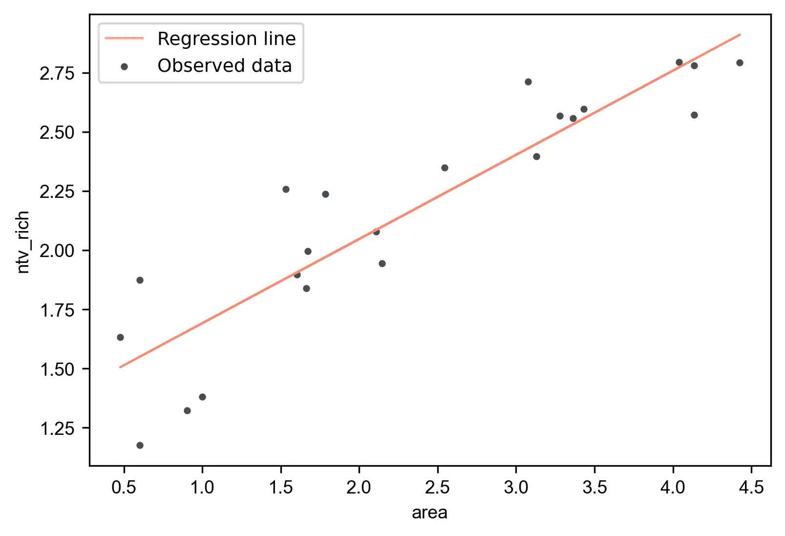
Regression plot
We have fitted the simple linear regression model with an equation [y = 1.3360 + (0.3557*area) ]. Now, generate
a regression plot for the fitted regression line.
from bioinfokit import visuz

# get predicted Y and add to original dataframe
df['yhat'] = reg.predict(X)
df.head(2)
   ntv_rich      area      yhat
0  1.897627  1.602060  1.905964
1  1.633468  0.477121  1.505779

# create regression plot with defaults
visuz.stat.regplot(df=df, x='area', y='ntv_rich', yhat='yhat')
# plot will be saved in same dir (reg_plot.png)
# set parameter show=True, if you want view the image instead of saving
Learn how to train linear regression model using neural networks (PyTorch)
Interpretation
- The regression line with
equation [
y = 1.3360 + (0.3557*area)] is helpful to predict the value of the native plant richness (ntv_rich) from the given value of the island area (area). - The p value associated with the
areais significant (p < 0.001). It suggests that the island area significantly influences native plant richness. - From the ANOVA F test, the p value is significant (p = 4.40e-09),
which suggests that there is a significant relationship between native plant richness and island area. The independent
variable (
area) can reliably predict the dependent (ntv_rich) variable. - The coefficient of determination (R-Squared or r2 score) is 0.828 (82.8%), which suggests that 82.8% of the variance in
ntv_richcan be explained byareaalone. Adjusted R-Squared is useful where there are multipleXvariables in the model.
Verify linear Regression asumptions
Residuals vs fitted (y_hat) plot: This plot used to check for linearity, variances and outliers in the regression data
# get residuals and standardized residuals and add to original dataframe
df['res'] = pd.DataFrame(reg.resid)
df['std_res'] = reg.get_influence().resid_studentized_internal
df.head(2)
# output
   ntv_rich      area      yhat   std_res       res
0  1.897627  1.602060  1.905964 -0.040767 -0.008337
1  1.633468  0.477121  1.505779  0.655482  0.127689

# create fitted (y_hat) vs residuals plot
visuz.stat.reg_resid_plot(df=df, yhat='yhat', resid='res', stdresid='std_res')
# plot will be saved in same dir (resid_plot.png and std_resid_plot.png)
# set parameter show=True, if you want view the image instead of saving
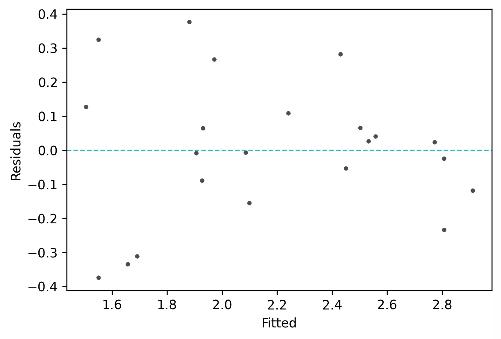
From the plot,
- As the data is pretty equally distributed around the line=0 in the residual plot, it meets the assumption of residual equal variances (homoscedasticity) and linearity. The outliers could be detected here if the data lies far away from the line=0.
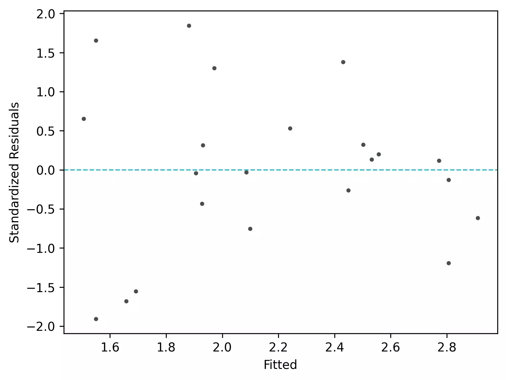
- In the standardized residual plot, the residuals are within -2 and +2 range and suggest that it meets assumptions of linearity
Quantile-quantile (QQ) plot: This plot used to check the data normality assumption
import statsmodels.api as sm
import matplotlib.pyplot as plt
# create QQ plot
# line=45 option to plot the data around 45 degree line
sm.qqplot(df['std_res'], line='45')
plt.xlabel("Theoretical Quantiles")
plt.ylabel("Standardized Residuals")
plt.show()
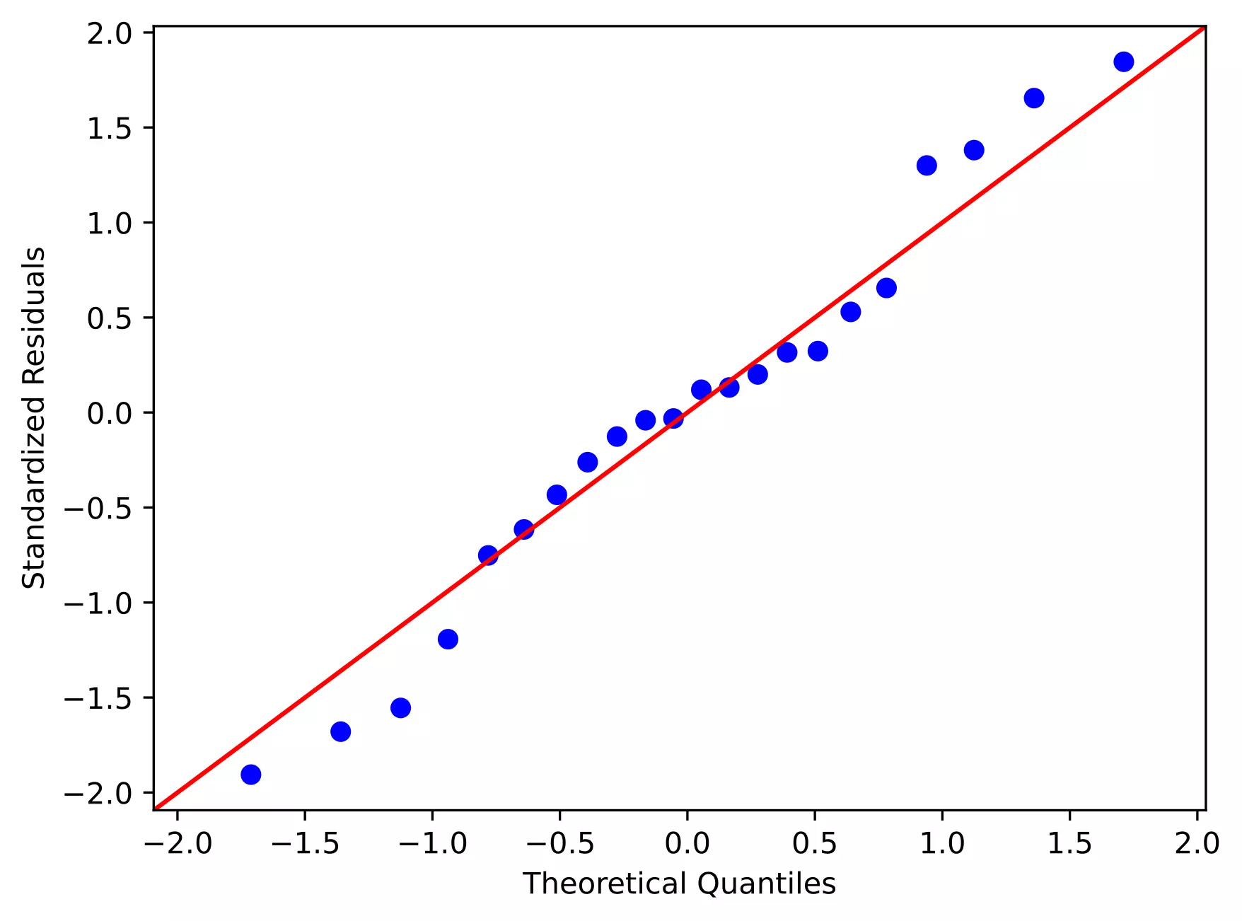
From the plot,
- As the standardized residuals lie around the 45-degree line, it suggests that the residuals are normally distributed
Enhance your skills with courses on regression and machine learning
- Machine Learning Specialization
- Linear Regression and Modeling
- Linear Regression with Python
- Linear Regression with NumPy and Python
- Building and analyzing linear regression model in R
- Machine Learning: Regression
- AI For Everyone
References
- Abdi H. Multiple correlation coefficient. Encyclopedia of measurement and statistics. 2007;648:651.
This work is licensed under a Creative Commons Attribution 4.0 International License
Some of the links on this page may be affiliate links, which means we may get an affiliate commission on a valid purchase. The retailer will pay the commission at no additional cost to you.

