Logistic regression in Python (feature selection, model fitting, and prediction)

What is logistic regression?
- Logistic regression models the binary (dichotomous) response variable (e.g. 0 and 1, true and false) as linear combinations of the single or multiple independent (also called predictor or explanatory) variables.
- Univariate logistic regression has one independent variable, and multivariate logistic regression has more than one independent variables.
- In logistic regression, the probability or odds of the response variable (instead of values as in linear regression) are modeled as function of the independent variables.
- For example, prediction of death or survival of patients, which can be coded as 0 and 1, can be predicted by metabolic markers.
Logistic regression assumptions
Logistic regression does not require to follow the assumptions of normality and equal variances of errors as in linear regression, but it needs to follow the below assumptions
- The linear relationship between the continuous independent variables and log odds of the dependent variable
- No multicollinearity among the independent variables. Multicollinearity can be tested using the Variance Inflation Factor (VIF).
- No influential outliers
- Independence of errors (residuals) or no significant autocorrelation. The residuals should not be correlated with each other. This can be tested using the Durbin-Watson test.
- The sample size should be large (at least 50 observations per independent variables are recommended)
Logistic regression model
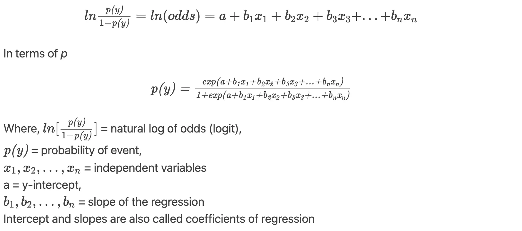
The logistic regression model follows a binomial distribution, and the coefficients of regression (parameter estimates) are estimated using the maximum likelihood estimation (MLE). The logistic regression model the output as the odds, which assign the probability to the observations for classification.
Odds and Odds ratio (OR)
- Odds is the ratio of the probability of an event happening to the probability of an event not happening (p ∕ 1-p). Odds can range from 0 to +∞.
- The odds ratio (OR) is the ratio of two odds. OR can range from 0 to +∞. OR is useful in interpreting the coefficients of regressions i.e effect of independent variables on the response variable, as coefficients of regressions would not be easy to interpret. OR can be obtained by exponentiating the coefficients of regressions.
Perform logistic regression in python
- We will use statsmodels, sklearn, seaborn, and bioinfokit (v1.0.4 or later)
- Follow complete python code for cancer prediction using Logistic regression
Note: If you have your own dataset, you should import it as pandas dataframe. Learn how to import data using pandas
from bioinfokit.analys import get_data
# get dataset for model training
df_train = get_data('wdbc_train').data
df_train.head(2)
        ID  dign  rad_mean  text_mean  peri_mean  area_mean  smooth_mean  comp_mean  conv_mean  conv_p_mean  sym_mean  frac_dim_mean
0  8711202     1     17.68      20.74     117.40      963.7      0.11150    0.16650    0.18550      0.10540    0.1971        0.06166
1   869218     0     11.43      17.31      73.66      398.0      0.10920    0.09486    0.02031      0.01861    0.1645        0.06562

# get test dataset
df_test = get_data('wdbc_test').data
Read my article on how to split train and test datasets in Python
- This dataset represents the characteristics of breast cancer cell nuclei computed from the digitized images (Dua and Graff 2019; Dr. William H. Wolberg, University Of Wisconsin Hospital at Madison).
- The features calculated from the digitized cell images include, radius, texture, perimeter, area, smoothness, compactness, concavity, concave points, symmetry, and fractal dimension for mean, standard error, and largest (worst) values. We have only used the mean values of these features (continuous variables) for regression analysis.
- The outcome (response variable) measured as malignant (1, positive class) or benign (0, negative class) (see dign variable in dataframe)
- Using the logistic regression model, I will build a classifier to predict the outcome as malignant or benign from given test samples
Check data distribution for the binary outcome variable,
# get count plot for the cancer outcome
import seaborn as sns
ax = sns.countplot(x='dign', data=df_train)
plt.show()
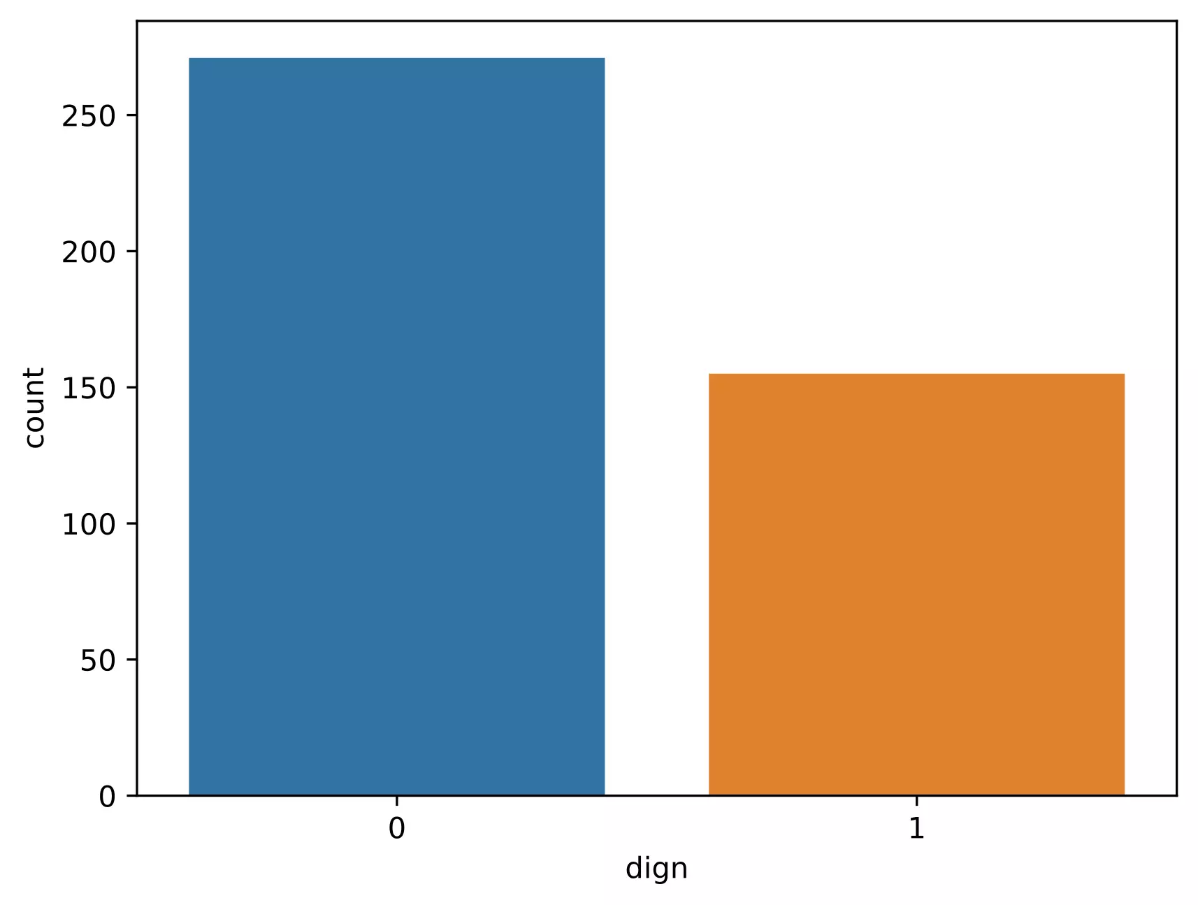
Note: It is crucial to have balanced class distribution, i.e., there should be no significant difference between positive and negative classes (commonly negative classes are more than positives in the life science field). The models trained on datasets with imbalanced class distribution tend to be biased and show poor performance toward minor class 4.
Feature selection for model training
- For good predictions of the regression outcome, it is essential to include the good independent variables (features) for fitting the regression model (e.g. variables that are not highly correlated). If you include all features, there are chances that you may not get all significant predictors in the model.
- Let’s visualize the data for correlation among the independent variables
from bioinfokit import visuz
X = df_train.iloc[:,2:12]
visuz.stat.corr_mat(df=X, cmap='RdBu')

- As you see in the correlation figure, several variables are highly correlated (multicollinearity) to each other (e.g. rad_mean and peri_mean). Multicollinearity can be an issue and reduce the performance of the fitted model. These spurious variables can be detected and dropped using various methods such the VIF, dimension reduction by PCA, recursive feature elimination (RFE), fitting models with all variables and removing insignificant variables, Chi-squared test etc.
- I have used the model fitting and to drop the features with high multicollinearity and insignificant variables.
- Based on model fitting and VIF analysis, I am using only text_mean, peri_mean, smooth_mean, conv_mean, and frac_dim_mean for the logistic regression analysis.
Logistic regression model fitting
# logistic regression model
import statsmodels.api as sm
# get independent variables
X = df_train[['text_mean',  'peri_mean', 'smooth_mean', 'conv_mean',  'frac_dim_mean']]
# to get intercept -- this is optional
# X = sm.add_constant(X)
# get response variables
Y = df_train[['dign']]
# fit the model with maximum likelihood function
model = sm.Logit(endog=Y, exog=X).fit()
# output message
Optimization terminated successfully.
         Current function value: 0.147065
         Iterations 10

print(model.summary())
# output
                           Logit Regression Results
==============================================================================
Dep. Variable:                   dign   No. Observations:                  426
Model:                          Logit   Df Residuals:                      421
Method:                           MLE   Df Model:                            4
Date:                Wed, 25 Nov 2020   Pseudo R-squ.:                  0.7757
Time:                        10:24:44   Log-Likelihood:                -62.650
converged:                       True   LL-Null:                       -279.29
Covariance Type:            nonrobust   LLR p-value:                 1.794e-92
=================================================================================
                    coef    std err          z      P>|z|      [0.025      0.975]
---------------------------------------------------------------------------------
text_mean         0.2511      0.060      4.204      0.000       0.134       0.368
peri_mean         0.0308      0.014      2.267      0.023       0.004       0.057
smooth_mean     103.0272     25.407      4.055      0.000      53.231     152.823
conv_mean        67.7988      8.614      7.871      0.000      50.916      84.682
frac_dim_mean  -387.2520     56.462     -6.859      0.000    -497.915    -276.589
=================================================================================

# get odds ratio
np.exp(model.params)
# output
text_mean         1.285496e+00
peri_mean         1.031256e+00
smooth_mean       5.547844e+44
conv_mean         2.783928e+29
frac_dim_mean    6.585474e-169
Interpretation
- The variable text_mean has an OR of 1.28 which suggests for one unit increase in text_mean we expect that about 1.28 times increase the odds of patient being malignant (assuming all other independent variables constant). Other independent variables can be interpreted in the same way.
- The p values for all independent variables are significant (p < 0.05) and suggests that these variables are highly associated with the outcome.
- Fractal dimension has a slight effect on cancer classification due to its very low OR
- The fitted model can be evaluated using the goodness-of-fit index pseudo R-squared (McFadden’s R2 index) which measures improvement in model likelihood over the null model (unlike OLS R-squared, which measures the proportion of explained variance). The pseudo R-squared value close to 1 suggests a better fitted model. However, it should be interpreted cautiously and other measures should also be considered for model evaluation. pseudo R-squared would be more useful when comparing the different models for similar datasets predicting the same outcome.
Prediction of test dataset using fitted model
# get the predicted values for the test dataset [0, 1]
pred = model.predict(exog=df_test[['text_mean',  'peri_mean', 'smooth_mean', 'conv_mean',  'frac_dim_mean']])
pred.head()
# output
0    0.004102
1    0.585947
2    0.999832
3    0.032939
4    0.000001

# predicted values > 0.5 classified as malignant (1) and <= 0.05 as benign (0)
round(pred)
0      0.0
1      1.0
2      1.0
3      0.0
4      0.0

# get confusion matrix and accuracy of the prediction
# note: there may be slightly different results if you use sklearn LogisticRegression method
from sklearn.metrics import accuracy_score, confusion_matrix
confusion_matrix(y_true=list(df_test['dign']), y_pred=list(round(pred)))
# output
array([[79,  7],
       [ 7, 50]], dtype=int64)

# fitted model accuracy
accuracy_score(y_true=list(df_test['dign']), y_pred=list(round(pred)))
# output
0.9020
Confusion matrix,
| Predicted Observed |
B(0) | M(1) |
|---|---|---|
| B(0) | 79 | 7 |
| M(1) | 7 | 50 |
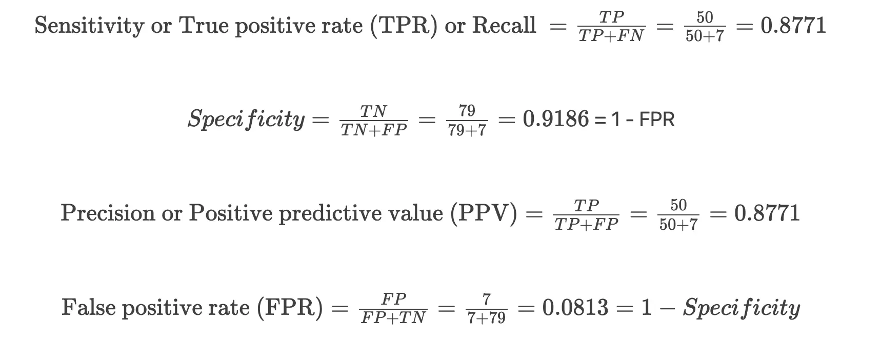
In the confusion matrix, diagonal numbers (79 and 50) indicates the correct predictions [true negatives (TN) and true positives (TP)] for the benign (0) and malignant (1) outcomes for test cancer datasets. The other numbers (7 and 7) indicates incorrect predictions [false positives (FP) and false negatives (FN)]
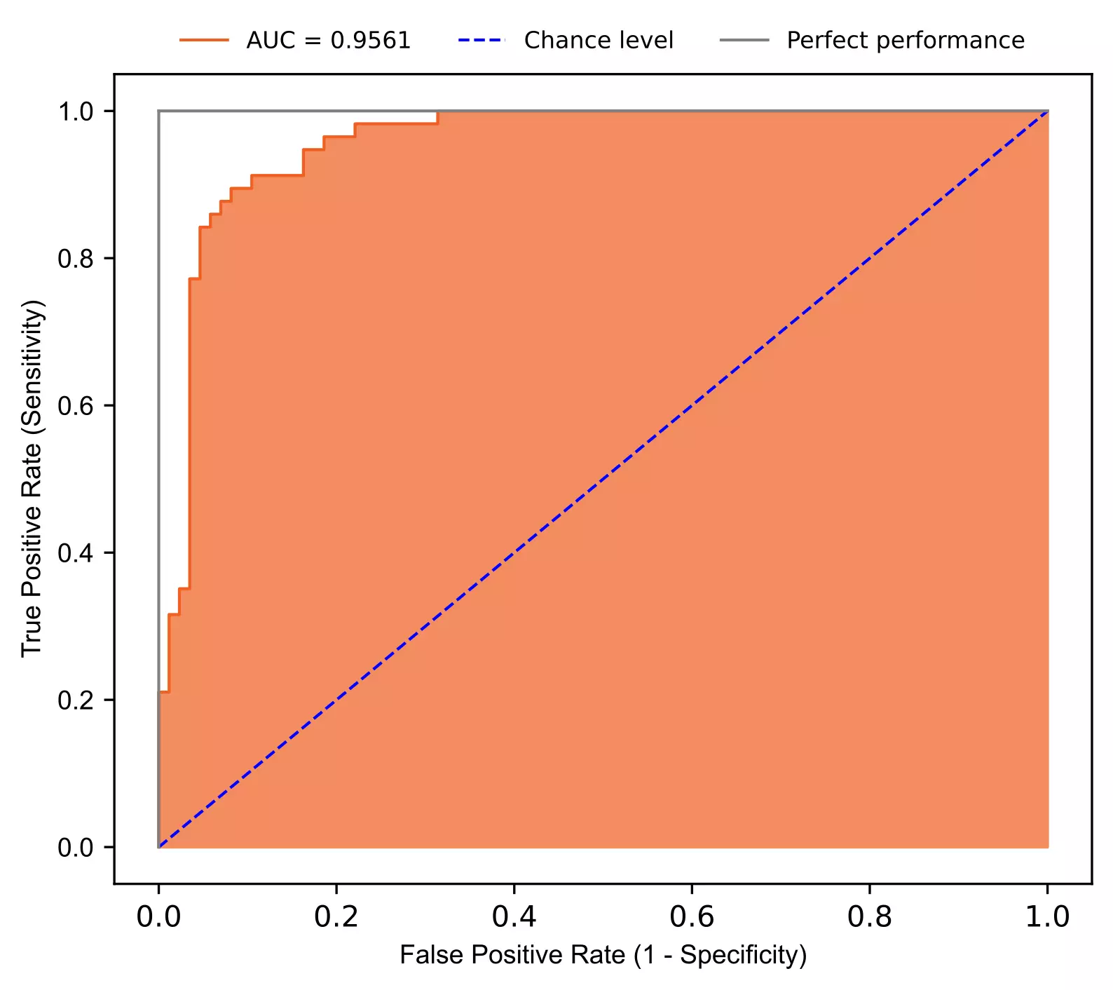
Plot Receiver Operating Characteristic (ROC) curve,
from sklearn.metrics import roc_curve, auc, roc_auc_score
from bioinfokit.visuz import stat

fpr, tpr, thresholds = roc_curve(y_true=list(df_test['dign']), y_score=list(pred))
auc = roc_auc_score(y_true=list(df_test['dign']), y_score=list(pred))
# plot ROC
stat.roc(fpr=fpr, tpr=tpr, auc=auc, shade_auc=True, per_class=True, legendpos='upper center', legendanchor=(0.5, 1.08), legendcols=3)
Interpretation
- In ROC, we can summarize the model predictability based on the area under curve (AUC). AUC range from 0.5 to 1 and a model with higher AUC has higher predictability. AUC refers to the probability that randomly chosen benign patients will have high chances of classification as benign than randomly chosen malignant patients.
- The fitted model has AUC 0.9561 suggesting better predictability in classification for breast cancer. The points lying above the chance level and close to grey line (perfect performance) represents a model with higher predictability.
- The accuracy of the fitted model is 0.9020. Even though accuracy is a measure of model performance, it is not alone enough. The AUC outperforms accuracy for model predictability. Two models can have the same accuracy but can differ in AUC. The models which are evaluated solely on accuracy may lead to misleading classification.
Related: Logistic regression in R
Enhance your skills with courses on Machine Learning
- Machine Learning Specialization
- Principal Component Analysis with NumPy
- Mathematics for Machine Learning: PCA
- Dimensionality Reduction in Python
- Python for Genomic Data Science
Related reading
- Support Vector Machine (SVM) basics and implementation in Python
- k-means clustering in Python [with example]
- Performing and visualizing the Principal component analysis (PCA) from PCA function and scratch in Python
References
- Dua, D. and Graff, C. (2019). UCI Machine Learning Repository [http://archive.ics.uci.edu/ml]. Irvine, CA: University of California, School of Information and Computer Science.
- Dr. William H. Wolberg, General Surgery Dept. University of Wisconsin, Clinical Sciences Center Madison, WI 53792
- Bewick V, Cheek L, Ball J. Statistics review 14: Logistic regression. Critical care. 2005 Feb 1;9(1):112.
- Hanley JA, McNeil BJ. The meaning and use of the area under a receiver operating characteristic (ROC) curve. Radiology. 1982 Apr;143(1):29-36.
- Smith TJ, McKenna CM. A comparison of logistic regression pseudo R2 indices. Multiple Linear Regression Viewpoints. 2013;39(2):17-26.
- Abdulhafedh A. Incorporating the multinomial logistic regression in vehicle crash severity modeling: a detailed overview. Journal of Transportation Technologies. 2017;7(03):279.
- Pearson RG, Thuiller W, Araújo MB, Martinez‐Meyer E, Brotons L, McClean C, Miles L, Segurado P, Dawson TP, Lees DC. Model‐based uncertainty in species range prediction. Journal of biogeography. 2006 Oct;33(10):1704-11.
- Josephat PK, Ame A. Effect of Testing Logistic Regression Assumptions on the Improvement of the Propensity Scores. Int. J. Stat. Appl. 2018;8:9-17.
If you have any questions, comments or recommendations, please email me at reneshbe@gmail.com
This work is licensed under a Creative Commons Attribution 4.0 International License
Some of the links on this page may be affiliate links, which means we may get an affiliate commission on a valid purchase. The retailer will pay the commission at no additional cost to you.

