RNA-seq Data Analysis with edgeR

Introduction
- Differential gene expression (DGE) analysis is commonly used in the transcriptome-wide analysis (using RNA-seq) for studying the changes in gene or transcripts expressions under different conditions (e.g. control vs infected).
- RNA sequencing (bulk and single-cell RNA-seq) using next-generation sequencing (e.g. Illumina short-read sequencing) is a de facto method for quantifying the transcriptome-wide gene or transcript expressions and performing DGE analysis.
- There are several computational tools are available for DGE analysis. In this article, I will cover edgeR for DGE analysis.
Check DGE analysis using DESeq2
DGE analysis using edgeR
The standard workflow for DGE analysis involves the following steps
- RNA-seq with a sequencing depth of 10-30 M reads per library (at least 3 biological replicates per sample)
- aligning or mapping the quality-filtered sequenced reads to respective genome (e.g. HISAT2 or STAR). You can read my article on how to map RNA-seq reads using STAR
- quantifying reads that are mapped to genes or transcripts (e.g. featureCounts, RSEM, HTseq)
- Actual raw integer read counts (un-normalized) are then used for DGE analysis using edgeR. edgeR prefers the raw integer read counts, but it can also work with expected counts obtained from RSEM.
Let’s start now for analyzing the gene expression data using edgeR,
Install edgeR
Install edgeR (follow this step if you have not installed edgeR before)
# R version 4.2.0 (2022-04-22 ucrt)
if (!require("BiocManager", quietly = TRUE))
    install.packages("BiocManager")

BiocManager::install("edgeR")
Import table of gene expression counts
Import the gene expression counts (read counts) as a matrix or a dataframe,
# load library
# edgeR version 3.38.0
library("edgeR")

# get count dataset
count_matrix <- as.matrix(read.csv("https://reneshbedre.github.io/assets/posts/gexp/df_sc.csv", row.names = "gene"))
# view first two rows
head(count_matrix, 2)
                 ctr1 ctr2 ctr3 trt1 trt2 trt3 length
Sobic.001G000200  338  324  246  291  202  168   1982
Sobic.001G000400   49   21   53   16   16   11   4769

# drop length column
count_matrix <- count_matrix[, -7]
head(count_matrix, 2)
                ctr1 ctr2 ctr3 trt1 trt2 trt3
Sobic.001G000200  338  324  246  291  202  168
Sobic.001G000400   49   21   53   16   16   11
Create DGEList data class
DGEList data class contains the integer count and sample information. DGEList is a list-based data object which is easy to manipulate in R.
Create a sample information for the count data,
sample_info <- c("ctr", "ctr", "ctr", "trt", "trt", "trt")
Now, create DGEList data class for count and sample information,
dge <- DGEList(counts = count_matrix, group = factor(sample_info))
dge
# output
An object of class "DGEList"
$counts
                 ctr1 ctr2 ctr3 trt1 trt2 trt3
Sobic.001G000200  338  324  246  291  202  168
Sobic.001G000400   49   21   53   16   16   11
Sobic.001G000700   39   49   30   46   52   25
Sobic.001G000800  530  530  499  499  386  264
Sobic.001G001000   12    3    4    3   10    7
15947 more rows ...

$samples
     group lib.size norm.factors
ctr1  ctr1  3356671            1
ctr2  ctr1  3184864            1
ctr3  ctr1  3292243            1
trt1  trt1  3141401            1
trt2  trt1  2719780            1
trt3  trt1  1762582            1
Filter out the genes with low counts
It is recommended to filter out the genes which have low expression counts across all samples. These genes may not have enough evidence for differential gene expression. The removal of low count genes also reduces the number of tests and ultimately multiple hypothesis testing corrections.
We will use the filterByExpr function to remove the low count genes. This function keeps the genes with a worthwhile
counts (at least 10 read counts) in a minimal number of samples. Here the minimal number of samples is 3 i.e. number of samples
in each group is 3.
keep <- filterByExpr(y = dge)

dge <- dge[keep, , keep.lib.sizes=FALSE]
# output
An object of class "DGEList"
$counts
                 ctr1 ctr2 ctr3 trt1 trt2 trt3
Sobic.001G000200  338  324  246  291  202  168
Sobic.001G000400   49   21   53   16   16   11
Sobic.001G000700   39   49   30   46   52   25
Sobic.001G000800  530  530  499  499  386  264
Sobic.001G001000   12    3    4    3   10    7
13828 more rows ...

$samples
     group lib.size norm.factors
ctr1   ctr  3343275            1
ctr2   ctr  3171392            1
ctr3   ctr  3278446            1
trt1   trt  3130360            1
trt2   trt  2709917            1
trt3   trt  1755290            1
Recalculating the library sizes (
keep.lib.sizes=FALSE) for each sample is recommended following the filtering step. After filtering, library sizes will be slightly changed for each sample.
Normalization and effective library sizes
edgeR normalizes the read counts for varying library sizes (sample-specific effect) by finding a scaling (normalization) factor for each sample. The normalization is performed using the TMM (Trimmed Mean of M-values) between-sample normalization method. TMM assumes most of the genes are not differentially expressed. The effective library sizes are then calculated by using the scaling factors.
calcNormFactors function is used for TMM normalization and calculating normalization
(scaling) factors
dge <- calcNormFactors(object = dge)
# output
An object of class "DGEList"
$counts
                 ctr1 ctr2 ctr3 trt1 trt2 trt3
Sobic.001G000200  338  324  246  291  202  168
Sobic.001G000400   49   21   53   16   16   11
Sobic.001G000700   39   49   30   46   52   25
Sobic.001G000800  530  530  499  499  386  264
Sobic.001G001000   12    3    4    3   10    7
13828 more rows ...

$samples
     group lib.size norm.factors
ctr1   ctr  3343275    1.0473246
ctr2   ctr  3171392    0.9815466
ctr3   ctr  3278446    1.0421847
trt1   trt  3130360    0.9837185
trt2   trt  2709917    0.9736776
trt3   trt  1755290    0.9744892
The normalization factors are an indicator of the status of gene expression. If the normalization factor is < 1 for some samples, it indicates a small number of high count genes are abundant in that sample and vice versa. The product of all normalization factors is equal to 1.
Model fitting and estimating dispersions
The edgeR uses the quantile-adjusted conditional maximum likelihood (qCML) method for single-factor design expression analysis. qCML method uses the pseudo count for adjusting the library sizes for all samples. edgeR internally calculates pseudo count for speeding up the analysis for negative binomial (NB) dispersion estimation and exact test for pairwise comparison.
The dispersion is estimated using estimateDisp() function. It estimates both common and tagwise dispersions in one
run.
dge <- estimateDisp(y = dge)
# output
An object of class "DGEList"
$counts
                 ctr1 ctr2 ctr3 trt1 trt2 trt3
Sobic.001G000200  338  324  246  291  202  168
Sobic.001G000400   49   21   53   16   16   11
Sobic.001G000700   39   49   30   46   52   25
Sobic.001G000800  530  530  499  499  386  264
Sobic.001G001000   12    3    4    3   10    7
13828 more rows ...

$samples
     group lib.size norm.factors
ctr1   ctr  3343275    1.0473246
ctr2   ctr  3171392    0.9815466
ctr3   ctr  3278446    1.0421847
trt1   trt  3130360    0.9837185
trt2   trt  2709917    0.9736776
trt3   trt  1755290    0.9744892

$common.dispersion
[1] 0.06972943

$trended.dispersion
[1] 0.05246027 0.10467010 0.09078381 0.05013202 0.12280665
13828 more elements ...

$tagwise.dispersion
[1] 0.03726749 0.08900702 0.05944770 0.02538477 0.21194794
13828 more elements ...

$AveLogCPM
[1] 6.507202 3.302021 3.883089 7.283077 1.570390
13828 more elements ...

$trend.method
[1] "locfit"

$prior.df
[1] 3.945552

$prior.n
[1] 0.9863879

$span
[1] 0.2950908
Testing for differential gene expression
After NB model fitting and dispersion estimation, the exact test (exact p values) is used for testing the differential expression of genes between two condition counts data.
The exact test is performed using the exactTest() function and is applied only on a single factor design. exactTest()
function outputs a DGEExact object containing the differential expression table (containing columns for log fold change,
logCPM, and two-tailed p values), comparison vector (comparing groups), and genes
data frame (gene annotation).
et <- exactTest(object = dge)
An object of class "DGEExact"
$table
                       logFC   logCPM     PValue
Sobic.001G000200 -0.01932342 6.507202 0.94991425
Sobic.001G000400 -1.04663708 3.302021 0.01929426
Sobic.001G000700  0.47456757 3.883089 0.17954409
Sobic.001G000800 -0.01486902 7.283077 0.94319628
Sobic.001G001000  0.59323937 1.570390 0.47828961
13828 more rows ...

$comparison
[1] "ctr" "trt"

$genes
NULL
topTags() function is useful to extract the table with adjusted p values (FDR). The output table is ordered by
p values.
top_degs = topTags(object = et, n = "Inf")
top_degs
# output
Comparison of groups:  trt-ctr
                      logFC    logCPM       PValue          FDR
Sobic.006G070564  5.1400611  3.308905 4.157243e-23 5.750715e-19
Sobic.003G079200  3.9750417  4.407321 4.527009e-21 3.131106e-17
Sobic.007G191200  3.8315481  6.609410 1.079306e-15 4.976681e-12
Sobic.010G095100  1.9839749  7.296541 1.905123e-15 6.588393e-12
Sobic.004G086500  4.1189965  4.615163 3.795766e-15 1.050137e-11
Sobic.004G222000  2.5899849  5.013418 1.395054e-14 3.216296e-11
Sobic.010G082600  4.6446796  3.485784 1.708966e-14 3.377162e-11
Sobic.004G121200  2.5401701  4.023315 2.491992e-14 4.308965e-11
.
.
As the comparison of groups is trt-ctr, the positive log fold change represents the gene is more highly expressed in the trt condition as compared to the ctr condition and vice versa.
Get a summary DGE table (returns significant genes with absolute log fold change at least 1 and adjusted p value < 0.05),
summary(decideTests(object = et, lfc = 1))
       trt-ctr
Down       177
NotSig   13367
Up         289
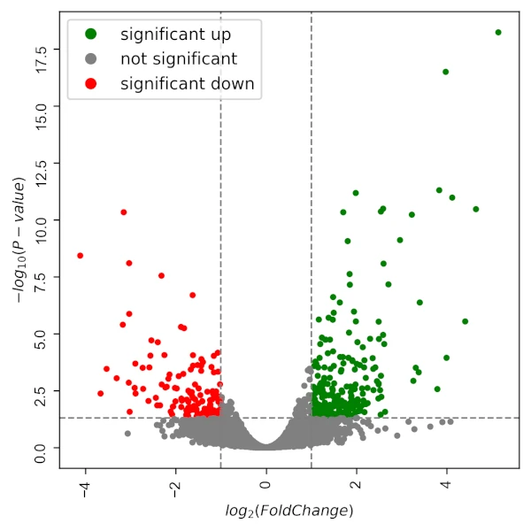
The differential gene expression of the sugarcane RNA-seq dataset suggests that 289 and 177 genes were significantly upregulated and downregulated respectively in response to the infected (trt) condition.
Export differential gene expression analysis table to CSV file,
write.csv(as.data.frame(top_degs), file="condition_infected_vs_control_dge.csv")
DGE Visualization
I will visualize the DGE using Volcano plot using Python,
Volcano plot,
# import packages
import pandas as pd
from bioinfokit import visuz

# import the DGE table (condition_infected_vs_control_dge.csv)
df = pd.read_csv("condition_infected_vs_control_dge.csv")
# drop NA values
df=df.dropna()

# create volcano plot
visuz.GeneExpression.volcano(df=df, lfc='logFC', pv='FDR', sign_line=True, plotlegend=True)
If you want to create a heatmap, check this article
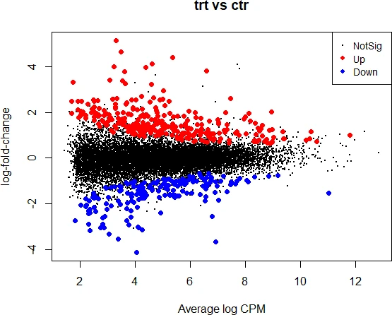
Visualize the MA plot,
plotMD(object = et)
Enhance your skills with courses on genomics and bioinformatics
- Genomic Data Science Specialization
- Biology Meets Programming: Bioinformatics for Beginners
- Python for Genomic Data Science
- Bioinformatics Specialization
- Command Line Tools for Genomic Data Science
- Introduction to Genomic Technologies
References
- Robinson MD, McCarthy DJ, Smyth GK. edgeR: a Bioconductor package for differential expression analysis of digital gene expression data. Bioinformatics. 2010 Jan 1;26(1):139-40.
- edgeR: differential analysis of sequence read count data
If you have any questions, comments or recommendations, please email me at reneshbe@gmail.com
This work is licensed under a Creative Commons Attribution 4.0 International License
Some of the links on this page may be affiliate links, which means we may get an affiliate commission on a valid purchase. The retailer will pay the commission at no additional cost to you.

