How to Perform ANOVA in Python

What is ANOVA (ANalysis Of VAriance)?

ANOVA is a statistical method used for analyzing the differences in means in three or more groups.

ANOVA compares the variance between-groups means to the variance within-groups. If the variance between-groups is larger than the within-groups, it suggests that there are differences in means among the groups.

Based on a number of independent variables (factors) and their groups, there are two main types of ANOVA viz. One-Way ANOVA and Two-Way ANOVA.

In One-Way ANOVA, there is one independent variable and two or more groups (levels). In Two-Way ANOVA, there are two independent variables, and each variable has two or more groups (levels).

ANOVA Hypotheses

• Null hypothesis: Groups means are equal (no variation in means of groups)
  H₀: μ₁=μ₂=…=μ_p
• Alternative hypothesis: At least, one group mean is different from other groups
  H₁: All μ are not equal

Note: The null hypothesis is tested using the omnibus test (F test) for all groups, which is further followed by post-hoc test to see individual group differences.

Learn more about hypothesis testing and interpretation

ANOVA Assumptions

• Assumption of normality: Residuals (experimental error) are approximately normally distributed (can be tested using Shapiro-Wilks test or histogram). Non-normality of the dependent variable can cause non-normality of residuals in ANOVA
• Homogeneity of variance (homoscedasticity): Variances of dependent variable are roughly equal between treatment groups (can be tested using Levene’s, Bartlett’s, or Brown-Forsythe test)
• Assumption of independence: Observations are sampled independently from each other (no relation in observations between the groups and within the groups) i.e., each subject should have only one response
• The dependent variable should be continuous. If the dependent variable is ordinal or rank (e.g. Likert item data), it is more likely to violate the assumptions of normality and homogeneity of variances. If these assumptions are violated, you should consider the non-parametric tests (e.g. Mann-Whitney U test, Kruskal-Wallis test).

ANOVA is a powerful method when the assumptions of normality and homogeneity of variances are valid. ANOVA is less powerful (little effect on type I error), if the assumption of normality is violated while variances are equal.

How ANOVA works?

• Check sample sizes: equal number of observation in each group
• Calculate Mean Square for each group (MS) (SS of group/level-1); level-1 is a degrees of freedom (df) for a group
• Calculate Mean Square error (MSE) (SS error/df of residuals)
• Calculate F value (MS of group/MSE)
• Calculate p value based on F value and degrees of freedom (df)

One-way (one factor) ANOVA

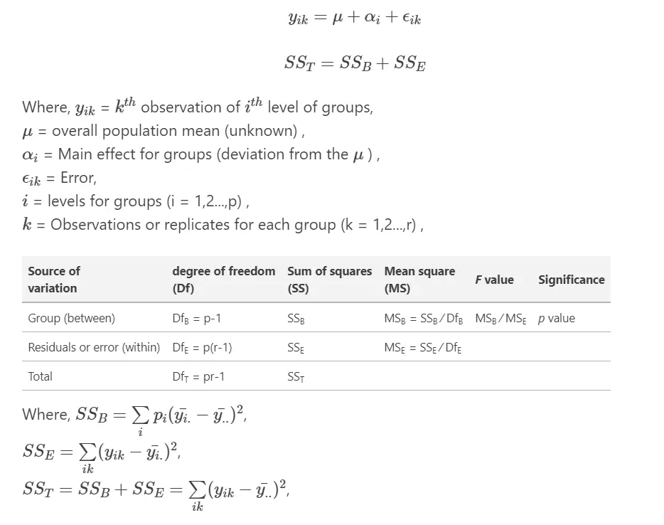
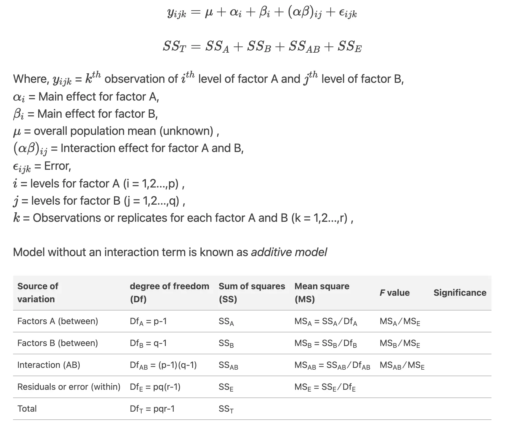
ANOVA effect model, table, and formula

The ANOVA table represents between- and within-group sources of variation, and their associated degree of freedoms, the sum of squares (SS), and mean squares (MS). The total variation is the sum of between- and within-group variances. The F value is a ratio of between- and within-group mean squares (MS). p value is estimated from F value and degree of freedoms.

ANOVA example

Example data for one-way ANOVA analysis tutorial, dataset

A	B	C	D
25	45	30	54
30	55	29	60
28	29	33	51
36	56	37	62
29	40	27	73

Here, there are four treatments (A, B, C, and D), which are groups for ANOVA analysis. Treatments are independent variable and termed as factor. As there are four types of treatments, treatment factor has four levels.

For this experimental design, there is only factor (treatments) or independent variable to evaluate, and therefore, one-way ANOVA method is suitable for analysis.

Note: If you have your own dataset, you should import it as pandas dataframe. Learn how to import data using pandas

import pandas as pd
# load data file
df = pd.read_csv("https://reneshbedre.github.io/assets/posts/anova/onewayanova.txt", sep="\t")
# reshape the d dataframe suitable for statsmodels package 
df_melt = pd.melt(df.reset_index(), id_vars=['index'], value_vars=['A', 'B', 'C', 'D'])
# replace column names
df_melt.columns = ['index', 'treatments', 'value']

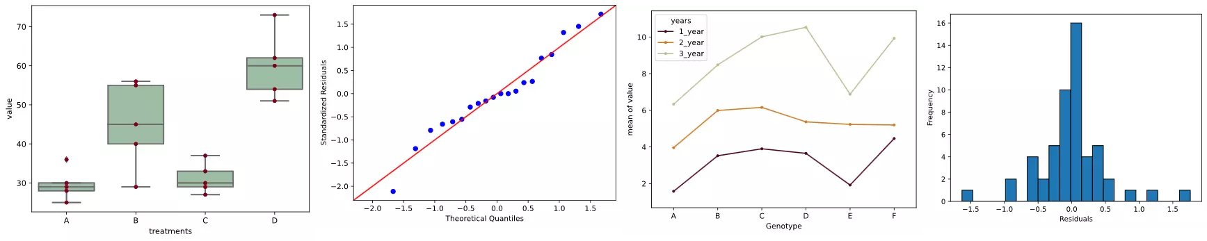
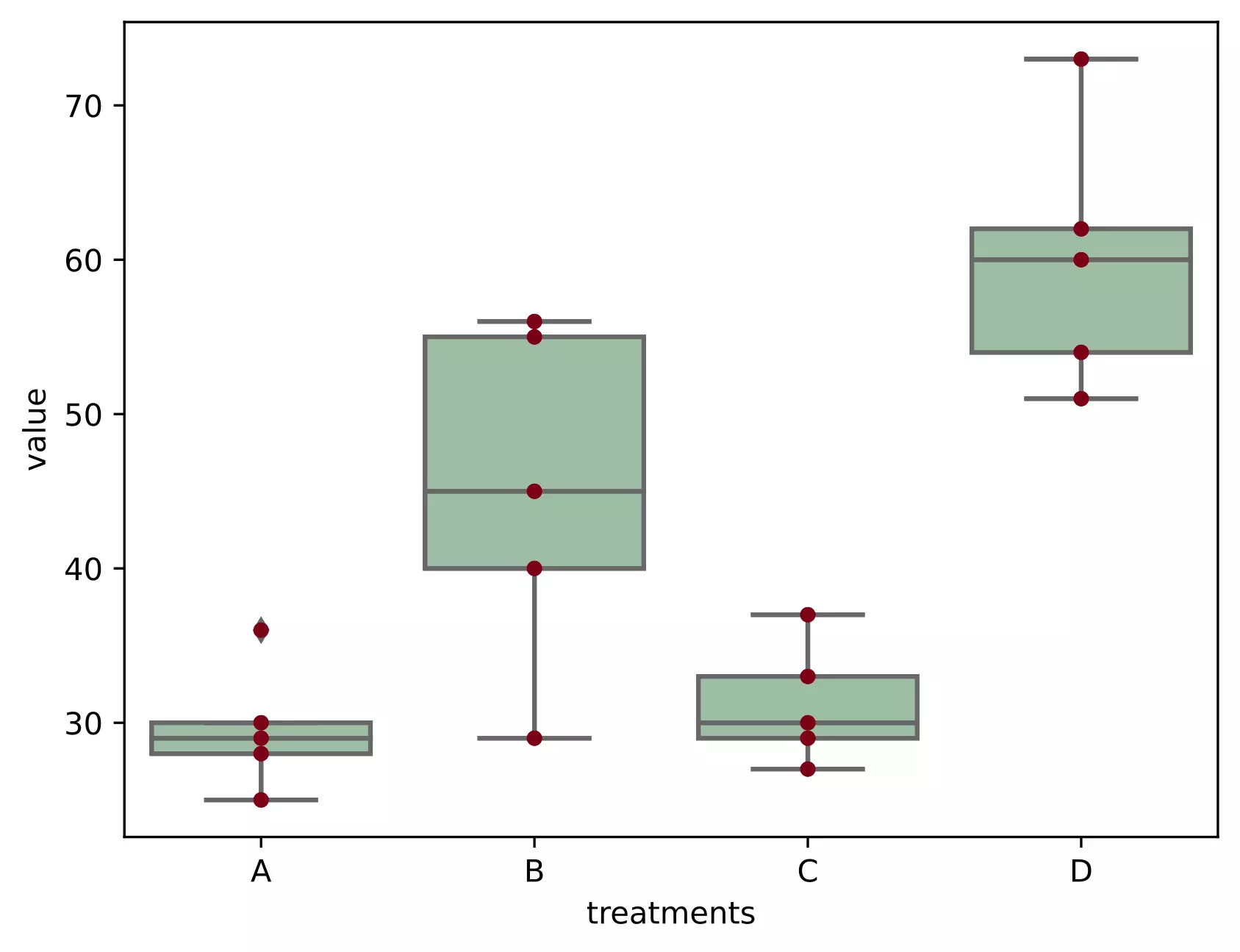
# generate a boxplot to see the data distribution by treatments. Using boxplot, we can 
# easily detect the differences between different treatments
import matplotlib.pyplot as plt
import seaborn as sns
ax = sns.boxplot(x='treatments', y='value', data=df_melt, color='#99c2a2')
ax = sns.swarmplot(x="treatments", y="value", data=df_melt, color='#7d0013')
plt.show()

import scipy.stats as stats
# stats f_oneway functions takes the groups as input and returns ANOVA F and p value
fvalue, pvalue = stats.f_oneway(df['A'], df['B'], df['C'], df['D'])
print(fvalue, pvalue)
# 17.492810457516338 2.639241146210922e-05

# get ANOVA table as R like output
import statsmodels.api as sm
from statsmodels.formula.api import ols

# Ordinary Least Squares (OLS) model
model = ols('value ~ C(treatments)', data=df_melt).fit()
anova_table = sm.stats.anova_lm(model, typ=2)
anova_table
# output (ANOVA F and p value)
                sum_sq    df         F    PR(>F)
C(treatments)  3010.95   3.0  17.49281  0.000026
Residual        918.00  16.0       NaN       NaN

# ANOVA table using bioinfokit v1.0.3 or later (it uses wrapper script for anova_lm)
from bioinfokit.analys import stat
res = stat()
res.anova_stat(df=df_melt, res_var='value', anova_model='value ~ C(treatments)')
res.anova_summary
# output (ANOVA F and p value)
                 df   sum_sq   mean_sq         F    PR(>F)
C(treatments)   3.0  3010.95  1003.650  17.49281  0.000026
Residual       16.0   918.00    57.375       NaN       NaN

# note: if the data is balanced (equal sample size for each group), Type 1, 2, and 3 sums of squares
# (typ parameter) will produce similar results.

Check how to calculate p value by hand

Interpretation

The p value obtained from ANOVA analysis is significant (p < 0.05), and therefore, we conclude that there are significant differences among treatments.

Note on F value: F value is inversely related to p value and higher F value (greater than F critical value) indicates a significant p value.

Note: If you have unbalanced (unequal sample size for each group) data, you can perform similar steps as described for one-way ANOVA with balanced design (equal sample size for each group).

From ANOVA analysis, we know that treatment differences are statistically significant, but ANOVA does not tell which treatments are significantly different from each other. To know the pairs of significant different treatments, we will perform multiple pairwise comparison (post hoc comparison) analysis for all unplanned comparison using Tukey’s honestly significantly differenced (HSD) test.

Note: When the ANOVA is significant, post hoc tests are used to see differences between specific groups. post hoc tests control the family-wise error rate (inflated type I error rate) due to multiple comparisons. post hoc tests adjust the p values (Bonferroni correction) or critical value (Tukey’s HSD test).

Tukey’s HSD test accounts for multiple comparisons and corrects for family-wise error rate (FWER) (inflated type I error)

Tukey and Tukey-kramer formula

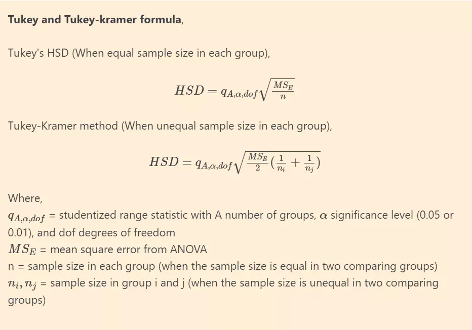
Alternatively, Scheffe’s method is completely coherent with ANOVA and considered as more appropriate post hoc test for significant ANOVA for all unplanned comparisons. However, it is highly conservative than other post hoc tests.

# we will use bioinfokit (v1.0.3 or later) for performing tukey HSD test
# check documentation here https://github.com/reneshbedre/bioinfokit
from bioinfokit.analys import stat
# perform multiple pairwise comparison (Tukey's HSD)
# unequal sample size data, tukey_hsd uses Tukey-Kramer test
res = stat()
res.tukey_hsd(df=df_melt, res_var='value', xfac_var='treatments', anova_model='value ~ C(treatments)')
res.tukey_summary
# output
  group1 group2  Diff      Lower      Upper   q-value   p-value
0      A      B  15.4   1.692871  29.107129  4.546156  0.025070
1      A      C   1.6 -12.107129  15.307129  0.472328  0.900000
2      A      D  30.4  16.692871  44.107129  8.974231  0.001000
3      B      C  13.8   0.092871  27.507129  4.073828  0.048178
4      B      D  15.0   1.292871  28.707129  4.428074  0.029578
5      C      D  28.8  15.092871  42.507129  8.501903  0.001000

# Note: p-value 0.001 from tukey_hsd output should be interpreted as <=0.001

Above results from Tukey’s HSD suggests that except A-C, all other pairwise comparisons for treatments rejects null hypothesis (p < 0.05) and indicates statistical significant differences.

Note: Tukey’s HSD test is conservative and increases the critical value to control the experimentwise type I error rate (or FWER). If you have a large number of comparisons (say > 10 or 20) to make using Tukey’s test, there may be chances that you may not get significant results for all or expected pairs. If you are interested in only specific or few comparisons and you won’t find significant differences using Tukey’s test, you may split the data for specific comparisons or use the t-test

Test ANOVA assumptions

• ANOVA assumptions can be checked using test statistics (e.g. Shapiro-Wilk, Bartlett’s, Levene’s test, Brown-Forsythe test) and the visual approaches such as residual plots (e.g. QQ-plots) and histograms.
• The visual approaches perform better than statistical tests. For example, the Shapiro-Wilk test has low power for small sample size data and deviates significantly from normality for large sample sizes (say n > 50). For large sample sizes, you should consider to use QQ-plot for normality assumption.

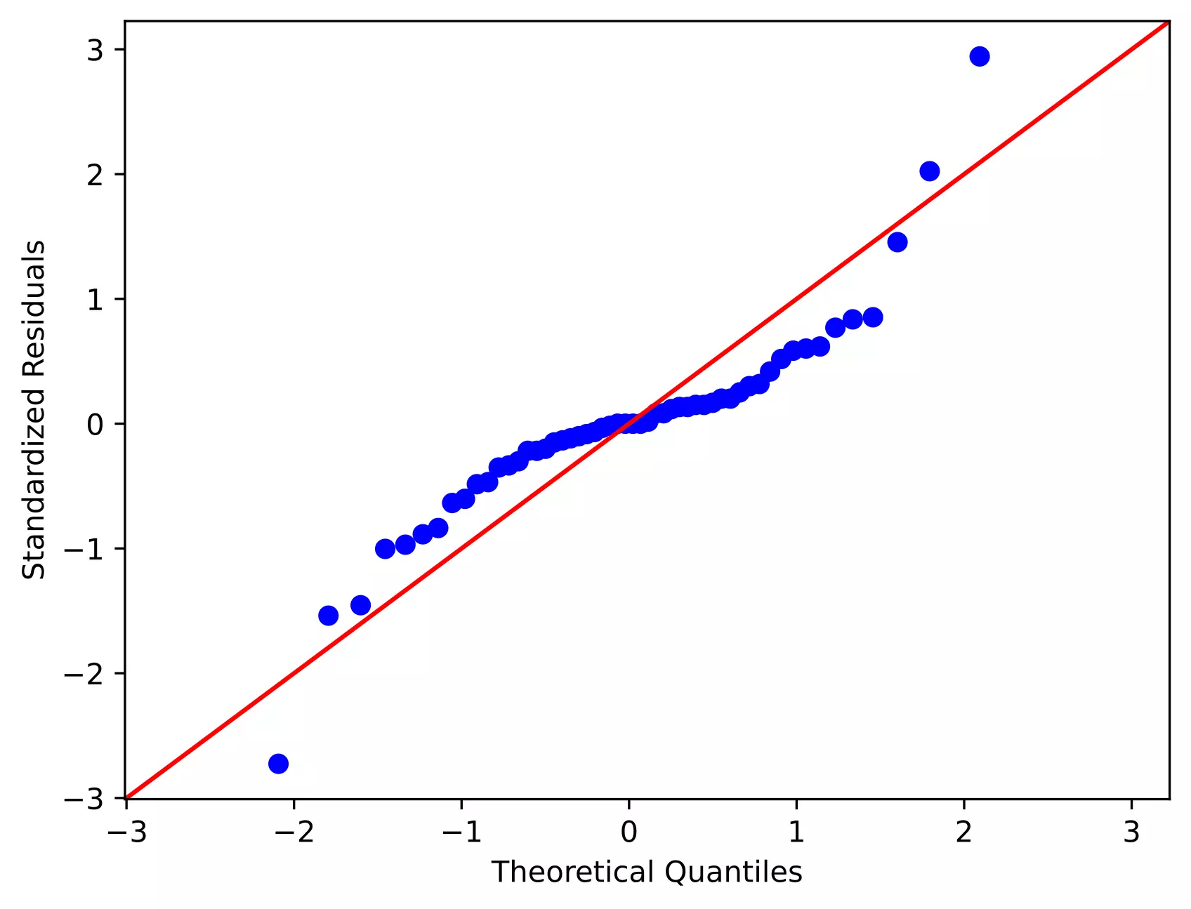
Now, I will generate QQ-plot from standardized residuals (outliers can be easily detected from standardized residuals than normal residuals)

# QQ-plot
import statsmodels.api as sm
import matplotlib.pyplot as plt
# res.anova_std_residuals are standardized residuals obtained from ANOVA (check above)
sm.qqplot(res.anova_std_residuals, line='45')
plt.xlabel("Theoretical Quantiles")
plt.ylabel("Standardized Residuals")
plt.show()

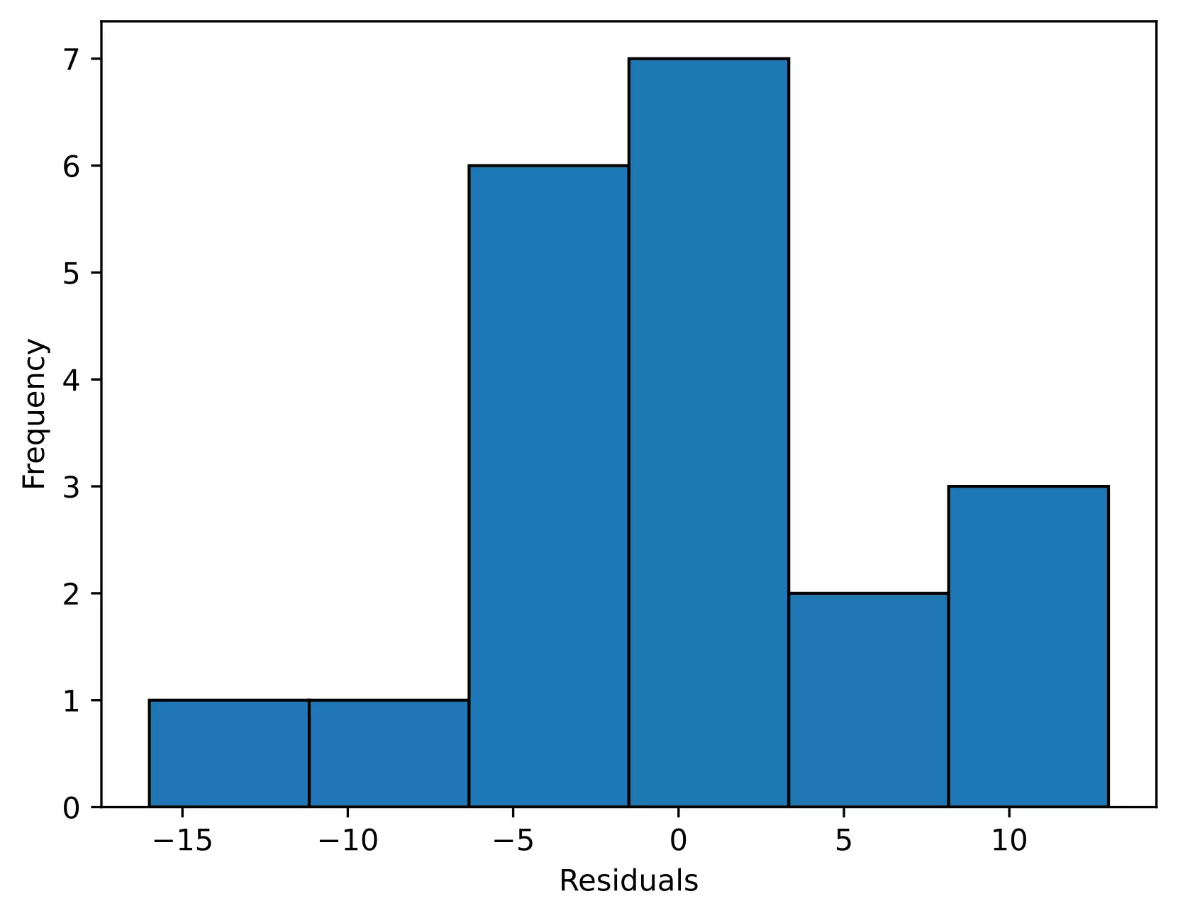
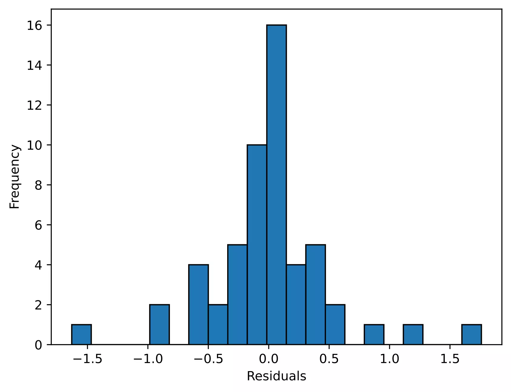
# histogram
plt.hist(res.anova_model_out.resid, bins='auto', histtype='bar', ec='k') 
plt.xlabel("Residuals")
plt.ylabel('Frequency')
plt.show()

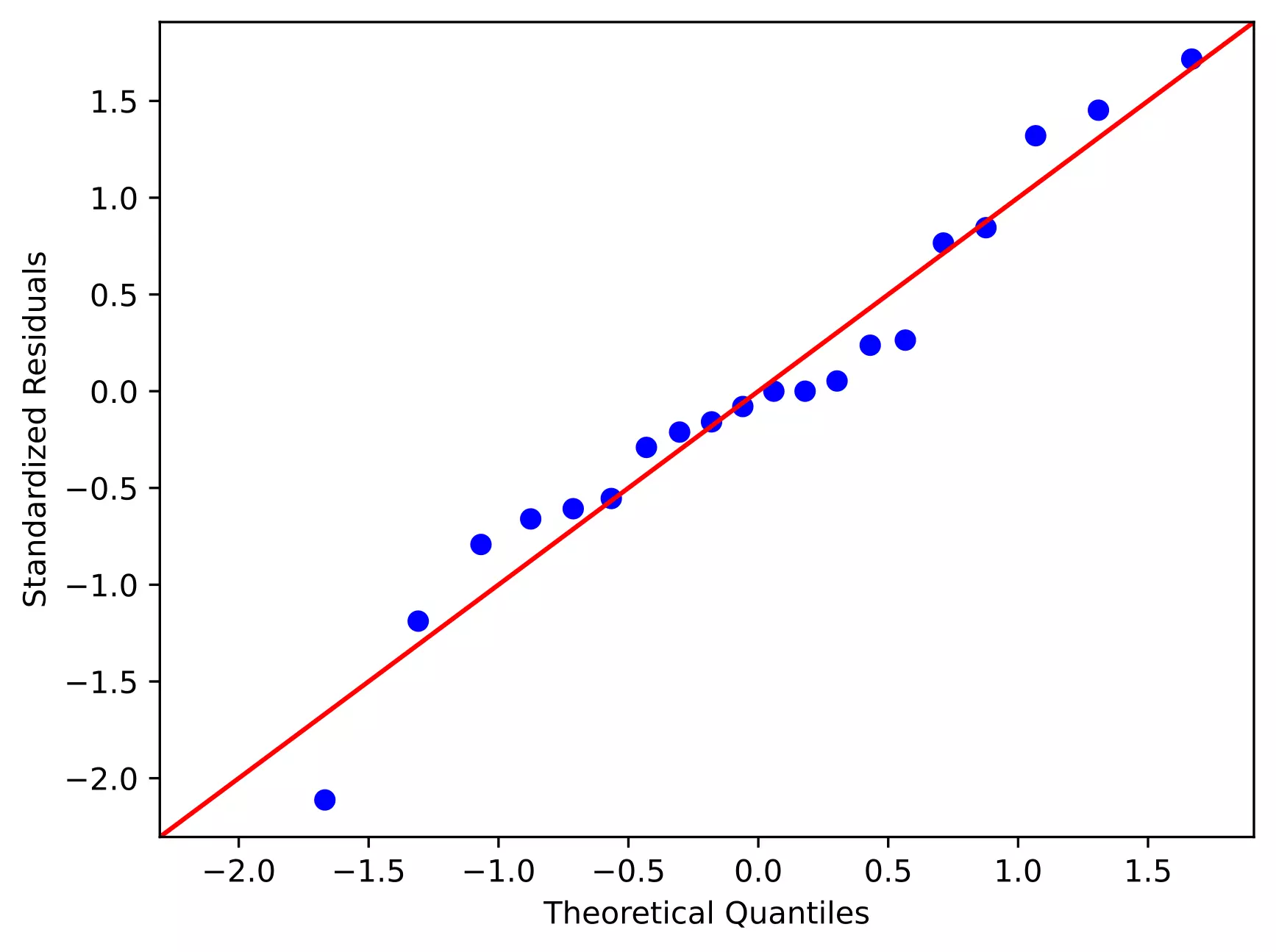
As the standardized residuals lie around the 45-degree line, it suggests that the residuals are approximately normally distributed

In the histogram, the distribution looks approximately normal and suggests that residuals are approximately normally distributed

Shapiro-Wilk test can be used to check the normal distribution of residuals. Null hypothesis: data is drawn from normal distribution.

import scipy.stats as stats
w, pvalue = stats.shapiro(model.resid)
print(w, pvalue)
# 0.9685019850730896 0.7229772806167603

As the p value is non significant, we fail to reject null hypothesis and conclude that data is drawn from normal distribution.

As the data is drawn from normal distribution, use Bartlett’s test to check the Homogeneity of variances. Null hypothesis: samples from populations have equal variances.

import scipy.stats as stats
w, pvalue = stats.bartlett(df['A'], df['B'], df['C'], df['D'])
print(w, pvalue)
5.687843565012841 0.1278253399753447

# if you have a stacked table, you can use bioinfokit v1.0.3 or later for the bartlett's test
from bioinfokit.analys import stat 
res = stat()
res.bartlett(df=df_melt, res_var='value', xfac_var='treatments')
res.bartlett_summary
# output
                 Parameter   Value
0      Test statistics (T)  5.6878
1  Degrees of freedom (Df)  3.0000
2                  p value  0.1278

As the p value (0.12) is non significant, we fail to reject null hypothesis and conclude that treatments have equal variances.

Levene’s test can be used to check the Homogeneity of variances when the data is not drawn from normal distribution.

# if you have a stacked table, you can use bioinfokit v1.0.3 or later for the Levene's test
from bioinfokit.analys import stat 
res = stat()
res.levene(df=df_melt, res_var='value', xfac_var='treatments')
res.levene_summary
# output
                 Parameter   Value
0      Test statistics (W)  1.9220
1  Degrees of freedom (Df)  3.0000
2                  p value  0.1667

Two-way (two factor) ANOVA (factorial design)

Here, I will discuss the two-way independent ANOVA, which differs from two-way mixed ANOVA and repeated measure ANOVA.

ANOVA factor effects model, table, and formula

Example data for two-way ANOVA analysis tutorial, dataset

From dataset, there are two factors (independent variables) viz. genotypes and yield in years. Genotypes and years has six and three levels respectively (see one-way ANOVA to know factors and levels).

For this experimental design, there are two factors to evaluate, and therefore, two-way ANOVA method is suitable for analysis. Here, using two-way ANOVA, we can simultaneously evaluate how type of genotype and years affects the yields of plants. If you apply one-way ANOVA here, you can able to evaluate only one factor at a time.

From two-way ANOVA, we can tests three hypotheses 1) effect of genotype on yield 2) effect of time (years) on yield, and 3) effect of genotype and time (years) interactions on yield

Note: If you have your own dataset, you should import it as pandas dataframe. Learn how to import data using pandas

import pandas as pd
import seaborn as sns
# load data file
d = pd.read_csv("https://reneshbedre.github.io/assets/posts/anova/twowayanova.txt", sep="\t")
# reshape the d dataframe suitable for statsmodels package 
# you do not need to reshape if your data is already in stacked format. Compare d and d_melt tables for detail 
# understanding 
d_melt = pd.melt(d, id_vars=['Genotype'], value_vars=['1_year', '2_year', '3_year'])
# replace column names
d_melt.columns = ['Genotype', 'years', 'value']
d_melt.head()
# output
  Genotype   years  value
0        A  1_year   1.53
1        A  1_year   1.83
2        A  1_year   1.38
3        B  1_year   3.60
4        B  1_year   2.94

As there are 6 and 3 levels for genotype and years, respectively, this is a 6 x 3 factorial design yielding 18 unique combinations for measurement of the response variable.

# generate a boxplot to see the data distribution by genotypes and years. Using boxplot, we can easily detect the 
# differences between different groups
sns.boxplot(x="Genotype", y="value", hue="years", data=d_melt, palette="Set3") 

import statsmodels.api as sm
from statsmodels.formula.api import ols
model = ols('value ~ C(Genotype) + C(years) + C(Genotype):C(years)', data=d_melt).fit()
anova_table = sm.stats.anova_lm(model, typ=2)
anova_table
# output
                          sum_sq    df           F        PR(>F)
C(Genotype)            58.551733   5.0   32.748581  1.931655e-12
C(years)              278.925633   2.0  390.014868  4.006243e-25
C(Genotype):C(years)   17.122967  10.0    4.788525  2.230094e-04
Residual               12.873000  36.0         NaN           NaN

# ANOVA table using bioinfokit v1.0.3 or later (it uses wrapper script for anova_lm)
from bioinfokit.analys import stat
res = stat()
res.anova_stat(df=d_melt, res_var='value', anova_model='value~C(Genotype)+C(years)+C(Genotype):C(years)')
res.anova_summary
# output
                        df      sum_sq     mean_sq           F        PR(>F)
C(Genotype)            5.0   58.551733   11.710347   32.748581  1.931655e-12
C(years)               2.0  278.925633  139.462817  390.014868  4.006243e-25
C(Genotype):C(years)  10.0   17.122967    1.712297    4.788525  2.230094e-04
Residual              36.0   12.873000    0.357583         NaN           NaN

Note: If you have unbalanced (unequal sample size for each group) data, you can perform similar steps as described for two-way ANOVA with the balanced design but set `typ=3`. Type 3 sums of squares (SS) does not assume equal sample sizes among the groups and is recommended for an unbalanced design for multifactorial ANOVA.

Interpretation

The p value obtained from ANOVA analysis for genotype, years, and interaction are statistically significant (p<0.05). We conclude that type of genotype significantly affects the yield outcome, time (years) significantly affects the yield outcome, and interaction of both genotype and time (years) significantly affects the yield outcome.

As the interaction is significant, let’s visualize the interaction plot (also called profile plot) for interaction effects,

from statsmodels.graphics.factorplots import interaction_plot
import matplotlib.pyplot as plt
fig = interaction_plot(x=d_melt['Genotype'], trace=d_melt['years'], response=d_melt['value'], 
    colors=['#4c061d','#d17a22', '#b4c292'])
plt.show()

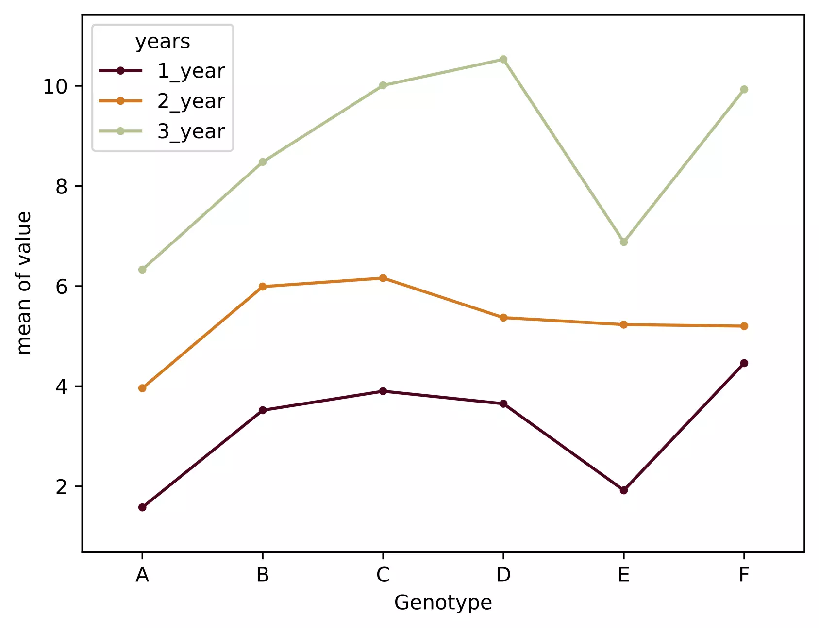
• The interaction plot helps to visualize the means of the response of the two factors (Genotype and years) on one graph. Generally, the X-axis should have a factor with more levels.
• From the interaction plot, the interaction effect is significant between the Genotype and years because three lines are not parallel (roughly parallel factor lines indicate no interaction - additive model). This interaction is also called ordinal interaction as the lines do not cross each other.
• For a more reliable conclusion of the interaction plot, it should be verified with the F test for interaction

Multiple pairwise comparisons (Post-hoc test)

Now, we know that genotype and time (years) differences are statistically significant, but ANOVA does not tell which genotype and time (years) are significantly different from each other. To know the pairs of significant different genotype and time (years), perform multiple pairwise comparison (Post-hoc comparison) analysis using Tukey’s HSD test.

# we will use bioinfokit (v1.0.3 or later) for performing tukey HSD test
# check documentation here https://github.com/reneshbedre/bioinfokit
from bioinfokit.analys import stat
# perform multiple pairwise comparison (Tukey HSD)
# unequal sample size data, tukey_hsd uses Tukey-Kramer test
res = stat()
# for main effect Genotype
res.tukey_hsd(df=d_melt, res_var='value', xfac_var='Genotype', anova_model='value~C(Genotype)+C(years)+C(Genotype):C(years)')
res.tukey_summary
# output
   group1 group2      Diff     Lower     Upper    q-value   p-value
0       A      B  2.040000  1.191912  2.888088  10.234409  0.001000
1       A      C  2.733333  1.885245  3.581421  13.712771  0.001000
2       A      D  2.560000  1.711912  3.408088  12.843180  0.001000
3       A      E  0.720000 -0.128088  1.568088   3.612145  0.135306
4       A      F  2.573333  1.725245  3.421421  12.910072  0.001000
5       B      C  0.693333 -0.154755  1.541421   3.478361  0.163609
6       B      D  0.520000 -0.328088  1.368088   2.608771  0.453066
7       B      E  1.320000  0.471912  2.168088   6.622265  0.001000
8       B      F  0.533333 -0.314755  1.381421   2.675663  0.425189
9       C      D  0.173333 -0.674755  1.021421   0.869590  0.900000
10      C      E  2.013333  1.165245  2.861421  10.100626  0.001000
11      C      F  0.160000 -0.688088  1.008088   0.802699  0.900000
12      D      E  1.840000  0.991912  2.688088   9.231036  0.001000
13      D      F  0.013333 -0.834755  0.861421   0.066892  0.900000
14      E      F  1.853333  1.005245  2.701421   9.297928  0.001000

# Note: p-value 0.001 from tukey_hsd output should be interpreted as <=0.001

# for main effect years
res.tukey_hsd(df=d_melt, res_var='value', xfac_var='years', anova_model='value ~ C(Genotype) + C(years) + C(Genotype):C(years)')
res.tukey_summary
# output
   group1  group2      Diff     Lower     Upper    q-value  p-value
0  1_year  2_year  2.146667  1.659513  2.633821  15.230432    0.001
1  1_year  3_year  5.521667  5.034513  6.008821  39.175794    0.001
2  2_year  3_year  3.375000  2.887846  3.862154  23.945361    0.001

# for interaction effect between genotype and years
res.tukey_hsd(df=d_melt, res_var='value', xfac_var=['Genotype','years'], anova_model='value ~ C(Genotype) + C(years) + C(Genotype):C(years)')
res.tukey_summary.head()
# output
        group1       group2  Diff     Lower     Upper    q-value   p-value
0  (A, 1_year)  (A, 2_year)  2.38  0.548861  4.211139   6.893646  0.002439
1  (A, 1_year)  (A, 3_year)  4.75  2.918861  6.581139  13.758326  0.001000
2  (A, 1_year)  (B, 1_year)  1.94  0.108861  3.771139   5.619190  0.028673
3  (A, 1_year)  (B, 2_year)  4.41  2.578861  6.241139  12.773520  0.001000
4  (A, 1_year)  (B, 3_year)  6.90  5.068861  8.731139  19.985779  0.001000

Test ANOVA assumptions

Similar to one-way ANOVA, you can use visual approaches, Bartlett’s or Levene’s, and Shapiro-Wilk test to validate the assumptions for homogeneity of variances and normal distribution of residuals.

# QQ-plot
import statsmodels.api as sm
import matplotlib.pyplot as plt
# res.anova_std_residuals are standardized residuals obtained from two-way ANOVA (check above)
sm.qqplot(res.anova_std_residuals, line='45')
plt.xlabel("Theoretical Quantiles")
plt.ylabel("Standardized Residuals")
plt.show()

# histogram
plt.hist(res.anova_model_out.resid, bins='auto', histtype='bar', ec='k') 
plt.xlabel("Residuals")
plt.ylabel('Frequency')
plt.show()

# Shapiro-Wilk test
import scipy.stats as stats
w, pvalue = stats.shapiro(res.anova_model_out.resid)
print(w, pvalue)
0.8978844881057739 0.00023986754240468144

Even though we rejected the Shapiro-Wilk test statistics (p < 0.05), we should further look for the residual plots and histograms. In the residual plot, standardized residuals lie around the 45-degree line, it suggests that the residuals are approximately normally distributed. Besides, the histogram shows the approximately normal distribution of residuals.

Note: The ANOVA model is remarkably robust to the violation of normality assumption, which means that it will have a non-significant effect on Type I error rate and p values will remain reliable as long as there are no outliers

We will use Levene’s test to check the assumption of homogeneity of variances,

# if you have  a stacked table, you can use bioinfokit v1.0.3 or later for the Levene's test
from bioinfokit.analys import stat 
res = stat()
res.levene(df=d_melt, res_var='value', xfac_var=['Genotype', 'years'])
res.levene_summary
# output
                 Parameter    Value
0      Test statistics (W)   1.6849
1  Degrees of freedom (Df)  17.0000
2                  p value   0.0927

As the p value (0.09) is non-significant, we fail to reject the null hypothesis and conclude that treatments have equal variances.

Enhance your skills with courses on ANOVA

• Statistics with Python Specialization
• ANOVA and Experimental Design
• Inferential Statistics
• Advanced Statistics for Data Science Specialization
• Introduction to Statistics

References

• Seabold, Skipper, and Josef Perktold. “statsmodels: Econometric and statistical modeling with python.” Proceedings of the 9th Python in Science Conference. 2010.
• Virtanen P, Gommers R, Oliphant TE, Haberland M, Reddy T, Cournapeau D, Burovski E, Peterson P, Weckesser W, Bright J, van der Walt SJ. SciPy 1.0: fundamental algorithms for scientific computing in Python. Nature methods. 2020 Mar;17(3):261-72.
• Mangiafico, S.S. 2015. An R Companion for the Handbook of Biological Statistics, version 1.3.2.
• Knief U, Forstmeier W. Violating the normality assumption may be the lesser of two evils. bioRxiv. 2018 Jan 1:498931.
• Kozak M, Piepho HP. What’s normal anyway? Residual plots are more telling than significance tests when checking ANOVA assumptions. Journal of Agronomy and Crop Science. 2018 Feb;204(1):86-98.
• Ruxton GD, Beauchamp G. Time for some a priori thinking about post hoc testing. Behavioral ecology. 2008 May 1;19(3):690-3.

Related reading

• How to perform one-way ANOVA in R
• How to perform two-way ANOVA in R

If you have any questions, comments, corrections, or recommendations, please email me at reneshbe@gmail.com

This work is licensed under a Creative Commons Attribution 4.0 International License

Some of the links on this page may be affiliate links, which means we may get an affiliate commission on a valid purchase. The retailer will pay the commission at no additional cost to you.